


APPENDIX 10.1 - METHODOLOGICAL ASPECTS
REFERENCE POPULATION AND POTENTIAL FOR IMPROVEMENT
Several road features have an influence on crash risk. Main rural roads, which are designed and operated following higher standards than those for secondary rural roads, are usually safer in terms of crashes per vehicle-km.
On any given road, the safety level is not constant. For example, crash densities are generally lower on links than at nodes, due to differences in the number of traffic conflicts. At nodes, T intersections are generally safer than + intersections for the same reason, and so on.
Consequently, the potential for improvement depends to a large extent on the nature of the site under study and on the modifications that can be envisioned.
Distinct reference populations should therefore be defined to help determine what constitutes a representative safety level for a given type of site. Such populations are defined by taking into account the main road features having an impact on safety. For example, a reference population may be defined for two-lane + intersections in urban areas with stops on the minor legs, another population for T intersections on similar roads, and so on. Given the significance of traffic flows with respect to crashes, distinct reference populations should ideally be developed for different combinations of traffic flows.
The establishment of reference populations requires a good knowledge of both crash contributing factors and available data that quickly limit the number of possible populations that can be defined. In practice, the development of statistical multivariate models is often used to circumvent data limitations.
RANDOM NATURE OF CRASHES
One of the main problems arising from the use of crash data to detect safety deficiencies has to do with the random nature of these events.
To make it easier to understand this concept and its consequences, let’s use a die as an analogy. A toss of the die is also a random event, whose result depends on the number of sides of the die and the value of each side. On a standard six-sided die, the range of possible values is simple: [1, 2, 3, 4, 5, 6]. When a die is thrown many times, each side should come up an equivalent number of times and the resulting mean value of such throws is 3.5: (1 + 2 + 3+ 4 + 5 + 6) / 6 = 3.5. This value can be described as the die's ‘long-term average’. When the die is thrown only a limited number of times, for example three times, the mean obtained may vary between extreme values of 1 and 6. If this result is used to estimate the die’s long-term average, accuracy will vary greatly. Similar variations also occur with crash frequencies. The number of crashes occurring at a site over a one-year period (f) can be compared to one throw of the die, while its long-term average crash frequency (m) can be compared to the die’s long-term average. From a statistical standpoint, the throwing of the die is said to follow a uniform distribution, while crashes follow a Poisson distribution.
Poisson distribution
where:
p(f;m) = probability of observing f crashes given that the safety level is m
f = crash frequency
m = safety level
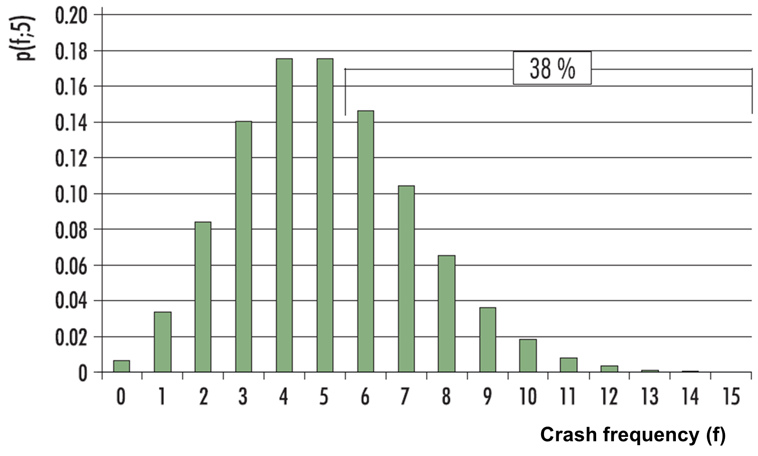
This is a fundamental equation in road safety analysis. It can be used to calculate the probability of a given crash frequency (f) when the safety level (m) is known. For example, if a site’s m value is 5 crashes/year, the probability of having exactly 1 crash/year is 3.4% while the probability of having 6 or more crashes is 38% (Figure 10.A1). The ‘Poisson test’ calculator can be used to calculate this latter probability.
Each site of a road network has its own ‘m’ value based on its set of characteristics (continuing the dice analogy, there would be several dice, each one with a distinct number of sides and values).
In practice, difficulties arise from the fact that the safety level (m) is unknown and that it must be estimated (m ̂) from the reported crash frequencies (f).
A calculator (CALCULATOR: CONFIDENCE INTERVAL ) is provided to estimate the uncertainty of ‘m’ based on an observed crash frequency.
This estimate of m becomes more statistically reliable as the period increases but it may be less representative of the prevailing conditions if changes have occurred at the site during the period considered. To avoid this type of bias, relatively short crash periods are often used (3 to 5 years).
REGRESSION TO THE MEAN
The regression to the mean phenomenon is common to a number of random events and consists of a general tendency for extreme values to return to median values. Sir Francis Galton, who noted that children of tall parents were usually shorter, and vice versa, was the first to identify regression to the mean in the 19th century (Galton, 1886). The phenomenon also applies to crashes. When the crash frequency is abnormally high during a certain period, it tends to decrease during the subsequent period and draw closer to the site’s long-term average (and vice versa).
SELECTION BIAS
The random nature of crashes and the difficulty of extending crash periods as much as might be necessary to reach sufficient accuracy create two types of biases during the identification phase, i.e. normal sites may be detected as being unsafe and unsafe sites may not be detected. Figure 10.A2 below, drawn from Hauer and Persaud (1984), illustrates the problem. The rectangle represents all the sites of a road network. Ellipsis 1 represents all the unsafe sites (those with a high ‘m’ value). It is solely at these sites that a treatment is warranted. Ellipsis 2 represents sites that were detected as being deviant during the identification phase (those with a high ‘f’ value). Four types of situations can arise (domains A to D):
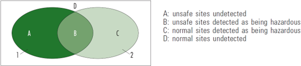
The objective of the identification stage is to obtain the best possible superimposition of ellipses 1 and 2 and to limit areas A and C. Identification techniques that take into account the random nature of crashes is seen to reduce selection bias.