APPENDIX 10.2 – PROCEDURES AND EXAMPLES
CRASH FREQUENCY
Procedure | Example (see Tables 10.A2 and 10.A3) |
|
|
|
|
where: frp = average crash frequency fj = crash frequency at site j of a reference population n = number of sites
| Two-lane rural roads Crash frequencies range from 0 to 14 crashes (Column 3 in Table A10.2.2)
frp = 258 crashes / 55 sites
IT = 2 x frp = 9.38 (9 crashes) Sections 1,10,12,45 and 52 are detected |
CRASH RATE
Procedure | Example (see Tables 10.A2 and 10.A3) |
|
|
|
|
where: Rj = crash rate of site j (crashes/Mveh-km) Rrp = average crash rate (crashes/Mveh-km) fj = crash frequency at site j P = period of analysis (years) Lj = section’s length of site j (km) Qj = average annual daily traffic of site j (AADT)
where: Rrp = average crash rate of (crash/Mveh-km) fj = crash frequency at site j P = period of analysis (years) Lj = section’s length of site j (km) Qw = weighted average annual daily traffic (AADT) Qj = AADT of site j
| Two-lane rural roads For section #1:
= 2.72 crashes/ Mveh-km Crash rates range from 0 to 4.73 crashes/Mveh-km (Column 4 in Table A10.2.2)
= 1.94 crashes/Mveh-km
IT = 2 x Rrp Sections 10, 33, 35 and 39 are detected |
Note: for intersections, L is not considered, and critical crash rates are expressed in terms of crashes/Mveh. | |
CRITICAL CRASH RATE
Procedure | Example (see Tables 10.A2 and 10.A3) |
|
|
|
|
| Two-lanes rural roads Column 4 in Table A10.2.2 For section #1: R1 = 2.72 crashes/Mveh-km Rrp = 1.94 crashes/Mveh-km |
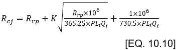 where: Rcj = critical crash rate at site j (crashes/Mveh-km) Rrp = average crash rate at similar sites (crashes/ Mveh-km) K = statistical constant: 1.036 for a level of confidence of 85% 1.282 for a level of confidence of 90% 1.645 for a level of confidence of 95% 2.326 for a level of confidence of 99% P = period of analysis (years) Lj = length of section j (km) Qj = average annual daily traffic at site j (AADT) | For section #1, with a level of confidence of 85%:
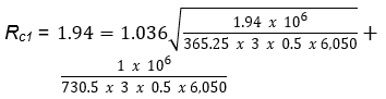 = 2.89 crashes/Mveh-km (Column 5 in Table A10.2.2) Critical crash rates range from 2.72 to 5.27 crashes/Mveh-km |
| Sections 10, 35 and 45 are detected (85% level of confidence) |
Note: for intersections, L is not considered, and critical crash rates are expressed in terms of crashes/Mveh. | |
CALCULATOR: CRITICAL CRASH RATE
EPDO
Procedure | Example (see Tables 10.A2 and 10.A3) |
|
|
|
|
| The weighting factors proposed by Agent (1973) are used in this example: 1.0 for property damage only crashes (PDO) |
EPDOj = where: EPDOj = equivalent property damage only index at site j wi = weighting factor for a crash severity i fij = frequency of a severity i crash at site j
where:
fj = total crash frequency at site j
| Two-lane rural roads For section #1:
EPDO1 = 2 x 9.5 + 3 x 3.5 + 4 x 1 = 33.5 Column 6 in Table A10.2.2 EPDO range from 0 to 33.5
Column 7 in Table A10.2.2
IT = 2 x IT = 2 x 2.16 = 4.32 Section 33 and 49 are detected |
RSI
Procedure | Example (see Tables 10.A2 and 10.A3) |
|
|
|
|
where: RSIj = relative severity index at site j fij = frequency of a type i crash at site j Ci= average cost of a type i crash
where: fj = total crash frequency of site j | Two-lane rural roads A cost grid must be developed, based on nationwide data. Values of Table 10.3 are used in this example. For section #1: RSI1 = (2 x $104,600) + (2 x $173,200) + (1 x $175,900) + (2 x $109,700) + (2 x $341,600) = $1,634,100
Columns 8 and 9 in Table A10.2.2 RSI range from $0 to $2,707,500
|
|
|
| IT = 2 x No section is detected by this criterion |
COMBINATION OF FREQUENCY AND RATE
Procedure | Example (see Tables 10.A2 and 10.A3) |
|
|
|
|
| Two-lane rural roads Columns 3 and 4 in Table A10.2.2 frp = 4.69 crashes per site Rrp = 1.94 crashes/Mveh-km Minimum investigation thresholds: 2 x frp and 2 x Rrp IT = 2 x frp = 2 x 4.69 = 9.38 crashes IT = 2 x Rrp = 2 x 1.94 = 3.88 crashes/Mveh-km According to this combination of criteria, section 10 warrants a detailed analysis |
BINOMIAL PROPORTION
Procedure | Example |
|
|
|
|
| Two-lane rural roads Surface conditions (reference population and section #45): Of the 12 crashes reported on section #45, 7 have occurred under wet-surface conditions (58%). The equivalent proportion in the reference population is 27%. 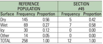 |
| For wet-surface conditions: The probability of observing 0, 1, ...6 wet surface crashes on section #45 and the corresponding cumulative distributions are shown in the table below. 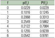 The probability of observing 6 or fewer wet-surface crashes is 98%. Consequently, the probability of observing 7 or more crashes is only 2% (i.e. the frequency of wet-surface crashes at the site is abnormally high). |
CRASH PREDICTION MODELS
Procedure | Example (see Tables 10.A2 and 10.A3) |
|
|
|
|
| Two-lane rural roads Columns 2 and 3 in Table A10.2.2 The following model has been fitted to the 55 sections of this example: fp = 0.0084 Q0,76 where: fp = predicted crash frequency / 3 years Q = average annual daily traffic (AADT) 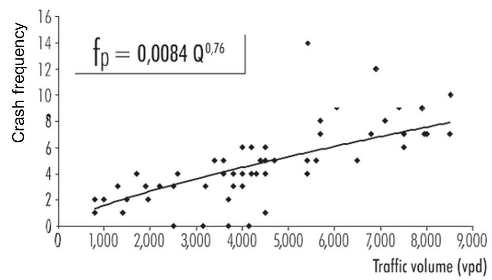 |
| For section 1: fp1 = 0.0084 × 60500,76 = 6.07 crashes/3 years Column 10 in Table A10.2.2 fp range from 1.31 to 7.84 crashes/3 years |
P.I.j = fj - fpj | For section 1: P.I.1 = 9-6.07 = 2.93 crash/3 years Column 11 in Table A10.2.2 P.I. range from 4.56 to 8.43 crash/3 years |
| Sections 10, 45, 1, 36 and 52 have the highest potential for improvement |
The following table presents a summary of the results obtained with the numerical example.
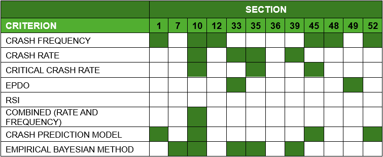
It shows that:
- Section 10 has been detected by 6 of these 8 identification criteria. Clearly, this section has a safety problem. When the problem is obvious, the choice of the identification criteria has less impact on the selection of sites.
- The crash frequency criterion detected mostly those sections with high traffic volumes (with the exception of section 10, every section detected has a daily traffic volume of more than 6,000 vehicles, while the average AADT is 4,400 vehicles). On the other hand, the crash rate criterion detected mostly sections with low traffic volumes (with the exception of section 10, every section detected has a daily traffic volume of fewer than 2,000 vehicles). This is a typical result for these criteria.
- Three criteria make direct use of the concept of potential for improvement to rank sections or its derivative: crash frequency, crash prediction model and empirical Bayesian (EB) methods. However, there are differences in the sections identified. Results obtained with the crash prediction model are deemed to be more reliable than those obtained with the crash frequency criterion as the estimate of the average crash frequency (reference population) is more accurate. Similarly, the result obtained using EB methods is seen to be more reliable than those obtained with the prediction model since it also improves the accuracy of the crash frequency at a site.
While definitive conclusions cannot be derived from an example, it nevertheless illustrates how the detection of sites may differ depending on the detection criterion used. For this reason, it is strongly recommended to make use of more than one identification criterion and to compare the obtained results.
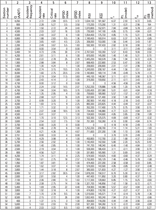
TABLE 10.A2: EXAMPLE – CRASH DATA (01/01/98 TO 31/12/00)
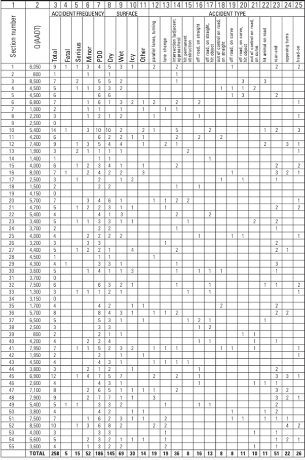
TABLE 10.A3: EXAMPLE – RESULTS