11.4 PRIORITY RANKING METHODS AND ECONOMIC ASSESSMENT
The previous chapter discussed how to identify risk, while the earlier part of this chapter discussed the use of effective interventions to address the risks that have been identified. The next important step is to determine the priority of different treatments. In most situations, there are likely to be financial constraints, which means that not all worthy projects or programmes can be funded. Therefore, a method is needed to identify which projects/programmes should be undertaken as the highest priority. There are also likely to be several options for addressing a risk, and it is necessary to see which of these options will produce the best safety benefit per unit cost. Economic appraisals or evaluations can be used to prioritise, compare and select road safety interventions. They help identify measures that yield the highest social return.
At the strategic level, it may also be necessary to establish the relative importance of proactive and reactive measures and decide on the budget proportion that will be allocated to each approach. The guidance provided in this chapter can be used at the strategic, programme or project level.
PIARC (2012) has produced the ‘State of the practice for cost-effectiveness analysis, cost-benefit analysis and resource allocation’ document, which provides comprehensive advice on methods to appraise projects and allocate resources. This document defines project appraisal as an assessment of the value of a project in order to establish whether the project meets the country’s economic and social objectives. Evaluation approaches include cost-effectiveness analysis (CEA) and cost-benefit analysis (CBA) (also referred to as benefit-cost analysis (BCA)). The outcome indicators from this analysis (BCR, NPV, FYRR and IRR) are discussed in Assessment Criteria. The following sections provide a summary of some of the key material on these issues.
Economic appraisal might prove to be challenging in some cases due to the lack of information regarding the Crash Modification Factors associated with a particular intervention or due to the difficulty in estimating the costs of the countermeasure. However, in the cases where the economic appraisal is possible, it provides a strong framework for the selection of the preferred countermeasures. The economic appraisal may be done through a cost-effectiveness analysis or a cost-benefit analysis.
Cost-effectiveness analysis involves comparing the cost of a proposed countermeasure with the outcome or effect it produces. Within cost-effectiveness, projects are ranked and screened according to their cost and effectiveness in improving road safety or achieving policy objectives. Cost-effectiveness is mainly applied when comparing alternative projects, programmes and policies with a similar outcome. This method can be utilised when monetising the benefits is not possible (e.g., due to lack of information on social costs of road crashes). The cost-effectiveness is expressed as the cost-effectiveness ratio (CER), which is calculated by dividing the number of crashes prevented by the cost of the measure. It can be defined as the number of crashes avoided per unit cost of implementing the measure.
Cost-benefit analysis uses monetary values to compare total benefits with total costs of any given policy, programme or project. It is mainly used to determine the worth of an investment based on the total benefits and costs of the investment, and to compare a project with any alternative projects. Cost-benefit analysis is used in road safety economic appraisal to help build a business case and secure funding for different projects or programmes. It enables comparisons between alternative road safety measures, identifying both the cost and the benefits to society to determine if the project should be undertaken and to establish priorities for approved projects. This, in turn, encourages the efficient allocation of limited resources to competing policies. Cost-benefit analysis requires assigning an economic value to the benefits, which can be done by determining the monetary value of the estimated crash reductions.
Yannis et al. (2008) provide a useful summary of cost-effective infrastructure interventions in an analysis for the Conference of European Directors of Roads (CEDR). They examined 55 road infrastructure investments, including reviews of both the costs and benefits of each. Based on this analysis, they identified several best practice examples that should be considered in the efficient planning of investments. The cost-effective intervention options were:
- Roadside treatments (clear zones and safety barriers).
- Speed limits.
- Junctions layout (roundabout, realignment, staggered junctions and channelisation).
- Traffic control at junctions (traffic signs and traffic signals).
- Traffic calming schemes.
DATA REQUIREMENTS
The key data requirements or parameters for estimating countermeasure benefits and costs are as follows:
INITIAL COST
Initial costs refer to implementation costs (e.g. installation, material and labour costs) for each countermeasure. The costs differ by road environment type, traffic volumes, local environment, local labour costs, and availability of materials. There is greater uncertainty surrounding implementation costs in most LMICs as the information is not readily available. The Road Safety Toolkit outlines general cost levels for different countermeasures. These values can be used as indicative measures where the treatments have not been implemented before or in cases where the cost information is not readily available.
ANNUAL MAINTENANCE AND OPERATING COSTS
Annual maintenance and operating costs refer to routine and periodic maintenance costs and running costs. The level and regularity of maintenance and associated operation costs depend on the countermeasure. As an example, junctions’ layout will most probably not require frequent maintenance, while markings and traffic signs will certainly require it.
TERMINAL SALVAGE VALUE
Some countermeasures may have a residual value if they are removed. For example, an intersection may be temporarily equipped with traffic signals for a number of years until a bypass is completed; after completion, the reduction in subsequent traffic flows may warrant the removal of the traffic signals. If the countermeasure asset can be used elsewhere, the recovery of this cost should be considered. However, in most cases, any residual value is likely to be negligible in the context of road safety countermeasures.
SERVICE/TREATMENT LIFE
A countermeasure’s service life refers to the time period over which a treatment will deliver safety benefits before major rehabilitation or replacement is required. It varies with:
- The type and scope of the project.
- Climate conditions (which may cause infrastructure deterioration).
- Traffic volumes (higher volumes might cause infrastructure deterioration, while growth in volumes may result in the need for different infrastructure).
- Local standards (more stringent construction requirements may result in slower deterioration).
- Resource and materials availability (certain materials are more resistant to deterioration).
- Regularity of maintenance.
For projects involving multiple treatments, e.g. intervention programmes on locations with high crash risk, the service life applied is that of the longest-lived component. Table 11.4 gives example maximum treatment lives for different countermeasures. Given the issues listed above, this is likely to vary substantially for individual projects. As an example, in the US, the treatment life for line-marking is expected to be one year, especially in States that experience snow and ice conditions.
| Treatment type | Recommended maximum treatment life (years) |
|---|---|
| Grade separation | 50 |
| Realign curve | 35 |
| Stagger or realign intersection | 35 |
| Roundabout | 30 |
| Median barrier | 30 |
| Shoulder sealing or widening | 25 |
| Add or widen lane (including overtaking lane) | 25 |
| Provide acceptable superelevation | 25 |
| Railway level crossing barriers | 20 |
| Median island (or other island) | 20 |
| Guardrail (roadside) | 20 |
| Street lighting | 20 |
| Remove roadside hazard (trees, pylons, etc.) | 20 |
| New traffic signals (hardware and/or software) | 15 |
| Improve sight distance by removing impediment on main road | 10 |
| Edge marker posts (guideposts) | 10 |
| Skid resistant surface | 10 |
| Signs (advisory, warning, parking, speed limit, etc.) | 10 |
| Raised reflectorized pavement markers | 5 |
| Line-marking (thermoplastic) | 5 |
| Line-marking (paint) |
Source: Adapted from Turner & Comport (2010).
ESTIMATE OF RESULTING CRASH CHANGES
The main benefits of road safety projects are expressed in terms of monetary savings from crash reductions or prevention of casualties (fatalities and injuries) over a given number of years.
Treatment effectiveness can be expressed as crash modification factors (CMFs). Several comprehensive resources that provide CMFs for different interventions are provided in Section 11.3 Intervention Options and Selection, including the CMF Clearinghouse database and the iRAP Road Safety Toolkit. As also discussed previously, the effectiveness and magnitude of crash changes can vary according to their context/environment.
In cases where several treatments are applied at the same location (multiple countermeasures), estimates of overall benefits need to be made. Some approaches have only included the crash savings from the primary or main treatment, but it is preferable that total benefits be calculated. Care needs to be taken to ensure that benefits are not counted more than once for interventions that improve safety in similar ways. For example, to address crashes at a curve, interventions such as advanced warning signs, audio-tactile edge lines, and improved road surface friction may be applied. The total benefit of these treatments will not equal the sum of benefits for each treatment, as each is alike in terms of its effect on crashes. For situations where treatments are linked, an adjustment needs to be made. Although several complex approaches have been devised to calculate the total benefit from multiple treatments, the simple approach outlined by Shen and Gan (2003) will usually suffice. They suggest a multiplicative formula similar in form to that shown below:
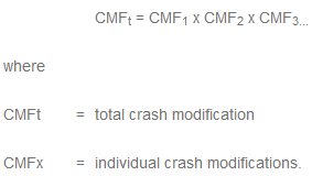
As an example, if three countermeasures are being considered in one location, with CMFs of 0.6, 0.75 and 0.8, the results would be as follows:
CMFt = 0.6 x 0.75 x 0.8
= 0.36, or 36% of crashes will remain (i.e. a 64% reduction in crashes)
A 64% reduction in casualties is obviously less than the 85% reduction that would be calculated if each reduction was added together.
Roberts and Turner (2007) were able to compare safety benefits at locations where packages of treatments were used, with locations where the same treatments were used but as single treatments. By applying the above formula, they identified that this approach tended to overestimate the true benefit of treatments. They suggested the results be multiplied by 0.66 to provide a more conservative approach (for the above example, this would produce a result of 42% reduction).
For a detailed discussion on the effectiveness of multiple treatment projects, see AASHTO (2025), iRAP (2013), and Elvik (2007).
MONETARY VALUES FOR DIFFERENT CATEGORIES OF ROAD CRASHES
The benefits resulting over time from safety countermeasures are estimated by placing an economic value on crashes and applying this to the expected reduction in crashes. Values should not be derived on a project-by-project basis but should be set at the national level and updated annually.
This economic value, referred to as the social cost of crashes, is the value of property damage caused by vehicle crashes, medical and ambulance costs, insurance and administration costs, loss of output costs, police costs, and human costs associated with the pain and suffering caused by death and injury. The different cost components are outlined in Table 11.5.
Costs per casualty |
Lost productivity (depending on the underlying hypothesis, gross loss of output or loss of output net of consumption) |
Human costs (loss of life expectancy, physical and mental suffering of the victim, mental suffering of the victim’s relatives and friends) |
Medical costs (medical rehabilitation) |
Non-medical rehabilitation |
Other economic costs. |
Costs per crash |
Damage to property (including environmental damage) |
Administration costs |
Other costs (e.g. congestion costs, vehicle rental costs). |
There have been many projects and considerable debate about the best way to determine crash costs (Hills & Jones-Lee, 1983; Alfaro et al., 1994; Jacobs, 1995), but it is now generally accepted that only two methods should be considered – the willingness-to-pay (WTP) approach and the human capital (HC) approach. These approaches are summarised in Table 11.6.
Approach | Description |
Human capital approach (HC) | Measures the impact of crash fatalities and injuries on present and future national output. The main attribute of HC is the present value of gross earnings (before tax). Direct costs such as vehicle costs, medical and emergency services costs are also added to the earnings estimate. In other cases, costs of human pain, suffering and grief are also included in the value of fatalities and injuries. |
The attributes can therefore be summarised as the value of future output loss due to casualties sustained in road crashes and the cost of resources spent to attend to the effects of the crashes. | |
Willingness-to-pay approach (WTP) | The estimates under the HC approach are average values rather than individual ones. |
Measures the amount individuals are willing to pay in order to reduce the risk of death and/or injury. Estimates are obtained from either revealed preferences (observing situations where individuals trade-off wealth or income for risk of death or injury) and stated preferences (individuals indicate how much they are willing to pay in order to reduce risk of death or injury based on hypothetical situations or questions). |
For a detailed description and discussion of the HC and WTP approaches, see PIARC (2012), HEATCO (2006), TRL (1995), and ADB (2005). Although both approaches are widely used, the willingness-to-pay (WTP) assessment method is generally recommended (DaCoTA, 2012; Harmon et al., 2018; McMahon & Dahdah, 2008).
Costs must be determined for crashes of varying levels of severity, usually fatal, serious, slight or minor, and property damage only. These severity levels can be defined as follows:
- A fatal crash results in the death of at least one person within 30 days of the crash.
- A serious crash does not result in any death, but at least one person has a severe injury such as fracture, internal injury, severe lacerations, etc. and must therefore be hospitalised.
- A minor crash does not result in any death or serious injury, but at least one person has a minor injury such as a cut, sprain or bruise.
- A property damage-only crash does not result in any injury or fatality, but damage to vehicles or property is sustained.
For the purpose of prioritising actions aimed at reducing crash frequency, a single average cost for all injury crashes is generally considered sufficient, particularly since it is difficult to predict the specific severities of crashes that might be prevented.
Costs are always based on average values, and in some countries, are also determined for broad road categories (e.g. urban, rural, freeway). The social cost of crashes provides an estimate of the economic burden that different crash and injury types place on the economy. For illustrative purposes, an example of costs by road category and crash severity for the UK in 2012 is shown in Table 11.7. These costs are updated annually and reported in the latest version of the report ‘Road Casualties Great Britain’ in Table RAS4001.
Costs increase from built-up roads to non-built-up roads to freeways, indicating the effect of greater speeds on crash severity levels. It can also be seen that there are approximately ten-fold increases in costs between severity levels. That is, the cost of a slight crash is about ten times that of a property damage-only crash, a serious crash is about ten times that of a slight crash, and a fatal crash is about ten times that of a serious crash.
| Cost per casualty UK £ (US$) | Cost per crash UK £ (US$) | |||
Crash/casualty type | All roads | Urban roads | Rural roads | Motorways | All roads |
Fatal | 2,411,659 (3,062,807) | 2,626,354 (3,335,470) | 2,800,894 (3,557,135) | 2,793,436 (3,547,664) | 2,718,861 (3,452953) |
Serious | 271,003 (344,173) | 300,810 (382,029) | 338,821 (430,303) | 344,914 (438,041) | 311,098 (395,095) |
Slight/minor | 20,892 (26,532) | 29,511 (37,479) | 36,394 (46,220) | 42,958 (54,557) | 31,132 (39,538) |
All injury crashes | 99,048 (125,790) | 109,897 (139,569) | 223,447 (283,778) | 165,385 (210,039) | 133,307 (169,300) |
Damage only | – – | 2,741 (3,481) | 4,007 (5,089) | 3,850 (4,890) | 2,880 (3,658) |
Calculation of crash costs is generally undertaken at the country level, and the development of an accurate figure can be a complex process regardless of which method is used. If no figure is available at the country level, a simple method for obtaining the value of crashes, especially in the absence of the data required for the HC and WTP approaches, is the iRAP ‘rule of thumb’ (McMahon & Dahdah, 2008). This method uses the information from countries that have already carried out WTP calculations, and analyses the relationship between the value of statistical life (VSL) and gross domestic product (GDP) per capita.
The recommendations for the economic appraisal model are to use (McMahon & Dahdah, 2008):
- A default value for statistical life of 70 times the GDP per capita (current price), with a range between 60 and 80 for sensitivity analysis.
- A default ratio of 10 serious injuries per fatality, with a range between 8 and 12 for sensitivity analysis.
- A default value of serious injury equivalent to 25% of the value of statistical life, with a range between 20% and 30% for sensitivity analysis.
The approach was originally developed using WTP values from a limited number of LMICs. These values were recently updated using a larger dataset (Milligan et al., 2014). The update showed that the rule of thumb tends to underestimate VSL for countries with GDP per capita above $7000 (Milligan et al., 2014).
Generation of crash costs can be a significant issue in LMICs, even with the availability of crash cost estimates, or when using the ‘rule of thumb’. Due to low GDP per capita in many countries, the crash costs can be low, while the cost of installing engineering treatments can remain high. The example (Box 11.2) below illustrates this issue using an example from Papua New Guinea.
BOX 11.2: POTENTIAL CRASH REDUCTIONS AND SAVINGS FROM IMPROVED ROAD MAINTENANCE IN PAPUA NEW GUINEA
In a study of the economic costs and benefits of alternative maintenance policies for the Highlands Highway in Papua New Guinea, comparisons were made between the highly responsive approach adopted in the Key Roads for Growth Maintenance Project (KRGMP) strategy, which was applied over the period 2006–2009, and alternative policies.
When compared with a ‘base option’ that involved minimum surface repairs only and had an almost six-month delay in response between the emergence of serious pavement defects and their repair; the combined NRRSP/KRGMP inputs, if continued over a twenty-year period, could deliver economic benefits of approximately K1.15 billion (approximately US$0.5 billion) with a marginal BCR of approximately 5, excluding crash cost savings. This resulted from prompt pavement repairs, with a monthly cycle of reactive surface maintenance, drainage and shoulder maintenance, and periodic resurfacing, and localised pavement repairs. Where the base option was changed to incorporate pavement strengthening or reconstruction when conditions were seriously deteriorated, the net benefits declined to between approximately K87 million and K629 million, with a maximum marginal BCR of 4.6.
Crash rates were also investigated and revealed a potential for reduction in crash risk by up to 30% from the current figures of approximately 4,000 casualties per year. This reduction was based on an assumed 15% reduction due to improved road surface condition, and a combination of factors such as improved visibility and shoulder conditions.
The total cost of crashes is given by the number of crashes of each type, multiplied by their unit cost of crashes. On this basis, the total cost of crashes is K24.4 million annually. To place this in proportion, it is equivalent to approaching a 2% reduction in all other costs; i.e. crash reductions will boost the cost saving due to improved maintenance by up to 2%.
The above figures are clearly impacted by the value of statistical life applied, noting that the value used is considerably less (by a factor of 42) than that applied in Australia. Furthermore, the relative crash rate for the Highlands Highway is approximately four times the base crash rate of typical Australian roads with similar operating conditions (McLean, 2001; Turner et al., 2009), which is not unexpected.
Consequently, the estimated gross crash costs are approximately 10% of those calculated for similar conditions in Australia. This is likely to have significant consequences for the economic justification of crash mitigation measures and warrants closer study.
Aspects that require consideration include: a) the value of statistical life, with the possibility that current ‘lost output’ methods take insufficient account of the extended family who are often supported by a ‘bread-winner’ in traditional societies in PNG and elsewhere. The loss of income has potential to affect the education and income-earning opportunities of a generation ; b) the need to account for real increases in income growth in LMICs, and the consequent increase in ‘real’ crash costs; c) the challenge of identifying affordable engineering treatments to mitigate crash risks, noting that the actual cost of road treatments delivered in LMICs and HICs are almost comparable (probably a maximum of 2 to 3 times different), whereas the value placed on the social cost of crashes is some 40 times less.
Alternatively, the value of different injury severities can be derived using Quality Adjusted Life Years (QALYs) and Disability Adjusted Life Years (DALYs). QALYs measure the value of a fatality prevented, taking into account the quantity and quality of life. They place a weight of one for a year of perfect health and zero for death. DALYs on the other hand, measure the quality of life lost or loss of life years due to illness or injury. They account for the burden of injury or illness and can also be used to measure property damage. DALYs and QALYs are widely used in health economics and very rarely in road safety. An example application of DALYs and QALYs in Colombia road safety is outlined in Box 11.3.
BOX 11.3 ESTIMATING THE COST OF CRASHES IN COLOMBIA
In estimating the cost of crashes in Colombia, Bhalla et al. (2013) applied the willingness to pay and the value of statistical life years methods. This involved estimating the incidence/occurrence and severity of injuries due to road crashes.
Using the well-established relationship between the value of statistical life and GDP per capita, they used different rules of thumb to estimate the cost of crashes using DALY estimates. These rules are outlined below.
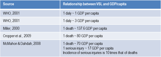
RELATIONSHIP BETWEEN VSL AND gdp CAPITAL (SOURCE: BHALLA ET AL., 2013)
The unit costs used in the estimation are outlined below.
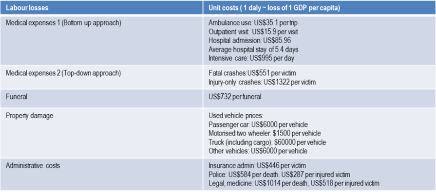
RELATIONSHIP BETWEEN VSL AND gdp CAPITAL LOSSES (SOURCE: BHALLA ET AL., 2013)
DISCOUNT RATE USED FOR SCHEMES
In any economic road project assessment, it is important to identify a base year from which all future costs and benefits can be assessed. This is because the value of a dollar received in the future is less than the value of a dollar now (also referred to as the ‘time value of money’). The discount rate is used to compare benefits and costs received at different points in time over a project’s treatment life, converting future benefits and costs to present values.
The choice of discount rate can have significant effects on the desirability and selection of projects, especially where benefits and costs accrue later in the treatment’s life. A higher discount rate reduces the value of benefits and costs occurring later in the treatment’s life, favouring projects where benefits occur early in the project. The World Bank recommends present value calculations at 12% discount rates (2014 values) be included in road project business case submissions (see PIARC, 2012; AASHTO, 2025). It is important to note, however, that this value is not necessarily relevant for every country, and the discount rate actually used can be significantly different. For instance, the discount rate is close to 5% in several western European countries.
ASSESSMENT CRITERIA
As indicated above, the standard approach for the ranking of treatments is to carry out a cost-benefit analysis, i.e. to compare the estimated benefits of each scheme (in terms of the value of crashes that will be prevented) in relation to its costs (implementation, maintenance, etc.). The treatments are then prioritised in accordance with the best economic returns.
As previously mentioned, estimating likely crash reductions resulting from remedial work is often difficult, because it can only be based on previous experience with similar schemes (Turner & Hall, 1994; Kulmala, 1994; Mackie, 1997).
The selection of countermeasure options is based on the first year rate of return (FYRR), the internal rate of return (IRR), the benefit-cost ratio (BCR), and the incremental benefit-cost ratio (IBCR), as well as net present value (NPV). The NPV is only used for complex projects, the FYRR is instead a fast method for comparing small projects. These measures indicate whether the benefits of the proposed treatment outweigh the costs, and if the preferred treatment has the greatest net social benefit.
It is worth pointing out that it is easy to have good indices with low-cost interventions, even if they save few lives. For this reason, the effectiveness of interventions in terms of the absolute number of crashes avoided should also be taken into account in the evaluation, and those with negligible effects should be excluded.
FIRST YEAR RATE OF RETURN (FYRR)
This is simply the net monetary value of savings and drawbacks anticipated in the first year of the scheme, expressed as a percentage of the total capital cost. The formula for calculating the FYRR is as follows:
where:
benefits = (crash savings in monetary terms) + (change in maintenance costs) + (change in journey costs)
Note that the last two elements of the benefits estimation might be considered to be small, particularly for low-cost schemes, and are often ignored.
This is not a rigorous evaluation criterion for prioritisation since it ignores any benefits or changes in maintenance costs after the first year. However, it is very simple to calculate, and given that road safety engineering schemes often produce first year rates of return in excess of 100%, more sophisticated decision criteria may not be necessary. This method usually yields high values with low-cost schemes but with relatively small crash savings, and for this reason it is less consistent with the Safe System approach.
The FYRR can also be used to assess the timing of a particular project by comparing it with the discount rate. If the FYRR is greater than the discount rate, the project can, in theory, proceed. This says nothing, however, of how it compares with other projects. If the FYRR is less than the discount rate, the project should, at the very least, be postponed.
More detailed assessments will be needed for schemes where crashes and traffic levels are expected to change substantially from year to year. For example, a scheme with an 80% FYRR may not be worthwhile if subsequent road closures due to the construction of a new road limit the benefit to just one year.
Example – First year rate of return (FYRR)
Example: a country has produced the road crash cost breakdown shown in Table 11.7. The average cost per crash is generally higher than the cost per casualty because, on average, there is more than one casualty in each crash. The average cost of an injury crash for 2023 has been calculated to be $125,790.
Now consider an intersection that had 12 injury crashes in 3 years, 9 of which involved right- angle collisions with drivers overshooting the stop line - this being the treatable group of crashes. Let us assume from past experience that the installation of a roundabout is likely to prevent two- thirds of these collisions. If the target FYRR for all schemes to be undertaken in the year in question has been set at 50%, then the maximum budget for the scheme may be calculated as:
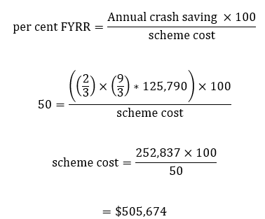
In other words, the scheme should not cost more than $505, 674 in order to achieve a 50% rate of return.
In the above example, the First Year Rate of Return has been used to determine the maximum cost of the scheme if a 50% rate of return is to be achieved. If the scheme did in fact cost $200,000, then the First Year Rate of Return would be more than 50% (actually 79%). This method could then be used to rank alternative schemes in order of their First Year Rate of Return.
Note: FYRR greater than 100% are need to make schemes economically viable
INTERNAL RATE OF RETURN (IRR)
Another important criterion used for assessing costs and benefits of highway schemes is the internal rate of return (IRR). This is the discount rate that makes the NPV equal to zero or makes the BCR equal to one. A theoretical example of how the discount rate affects the NPV of a project is shown in Figure 11.8.
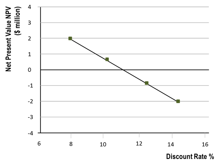
At discount rates of 8% or 10%, the project has a positive NPV, while it is negative at 12% or 14%. The NPV is zero at 11% discount rate, which is known as the internal rate of return (IRR). The IRR is preferred by multilateral aid agencies, such as the World Bank, because it avoids the use of local discount rates which, depending on their value, can significantly affect the NPV or NPV/PVC ratio.
The IRR provides a guideline to evaluate if a particular project or investment should be pursued. If the IRR is greater than the minimum required rate of return or hurdle rate (normally the cost of capital), then the project or investment can be worth pursuing as it is expected to generate returns greater than the cost of financing it. If the IRR is equal to the hurdle rate, the project is expected to break even with returns equivalent to the cost of capital. On the contrary, if the IRR is lower than the hurdle rate, then it is recommended to reject the project or investment, as the expected returns would be less than the costs of financing.
The internal rate of return (IRR) is useful to determine the profitability and attractiveness of a particular investment. Among different alternatives, the one with the highest IRR is preferable, provided that it is above the hurdle rate. The IRR can be used along other metrics such as the NPV to form a holistic view of the viability of a certain road safety project or investment.
BENEFIT-COST RATIO (bcr) AND INCREMENTAL BENEFIT-COST RATIO (IBCR)
Benefit cost ratio (BCR) is defined as the present value of benefits (PVB) divided by the present value of costs (PVC):
When the NPV of any given project is positive, the BCR is greater than one. The greater the BCR, the higher the benefits are. The BCR is used to rank projects where there is a budget constraint, and it serves as an indicator of a project’s economic efficiency.
The IBCR involves ranking a pairwise comparison of all alternatives with a BCR greater than one in order to determine the marginal benefit obtained for a marginal increment in cost. Then, after eliminating all schemes with a BCR of less than one, the schemes are listed in order of ascending cost and the marginal BCR is determined by a pairwise comparison of alternatives, starting with the lowest and second-lowest cost alternatives. That is:
where:
x and x+1 = the lowest and next to lowest cost alternatives
n = service life of the scheme
i = discount rate
x / x+1 =alternative x compared to alternative x+1
If the IBCR is greater than one, the alternative x+1 is preferred, since the marginal benefit is greater than the marginal cost. Conversely, if the IBCR is less than one, alternative x is preferred. The preferred option is then taken and the pairwise comparison is continued until only a single alternative remains, which should then be the most economically desirable of all the options considered.
NET PRESENT VALUE (NPV)
This type of evaluation expresses the difference between discounted costs and benefits of a scheme, which may extend over a number of years. As stated earlier, future benefits must be adjusted or discounted before being summed to obtain a present value. Changes may also take place over the life of the scheme which will affect benefits in future years.
Let us assume (for ease of calculation) that the current rate used by the government for highway schemes is 10%, which in the prevailing economic climate might be considered as somewhat high in most countries. This means that $100 in benefits accruing this year will be worth 10% less if it accrues next year. A further year's delay will reduce the benefit again, and so on. These figures can be summed over the life of the scheme to obtain the present value of benefits (PVB).
The equation below is used to calculate discount factors and resulting factors are shown in Appendix 11.1:
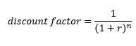
where:
r = discount rate
n = number of years
Net Present Value (NPV) is defined as the difference between the discounted monetary value of all the benefits and costs of a particular project or measure. The NPV is expressed as the PVB minus the PVC. A positive NPV indicates an improvement in economic efficiency compared with the base case.
With respect to implementation priorities, the economic criteria for scheme assessment using the NPV approach are:
- All schemes with a positive NPV are worthwhile in economic terms.
- For a particular site, the most worthwhile option is the one with the highest NPV.
Care needs to be taken in using NPV as the only investment criterion, since it tends to indicate projects with higher costs.
Example – NPV assessment
Let us assume that the anticipated initial cost of redesigning an intersection will be $200,000 spread out equally over two years, with annual maintenance costs over the next 5 years (the life of the scheme) of $8,000. Assume the discount rate to be 10%.
As noted above, the benefits are always difficult to estimate and will often require an educated guess. In this example, let us assume, based on previous experience in similar circumstances, that 10 injury crashes over the first two years (5 per year) will be saved, and that this will drop to 3 per year afterwards due to changes in traffic. If the average cost of an injury crash is $125,790, as shown in Table 11.7, the total savings would amount to $628 950 in each of the first two years, followed by $377,370 in each of the remaining 3 years. The Net Present Value is calculated in Table 11.8 to be $1,478,313.
TABLE 11.8: costs and benefits at a treated site
YEAR | DISCOUNT FACTOR | COST ($) | BENEFIT ($) | NET COST (-) OR BENFIT (+) ($) | NPV of Cost(-) OR Benefit (+) ($) |
|---|---|---|---|---|---|
(1) | (2) | (3) | (4) | (5)= (4)-(3) | (6)=(5)x(2) |
0 | 1.000 | 100,000 |
| -100,000 | -100,000 |
|
|
|
|
| |
1 | 0.909 | 100,000 |
| -100,000 | -90,909 |
Installation complete | |||||
2 | 0.826 | 8,000 | 626,950 | +620,950 | +512,905 |
3 | 0.751 | 8,000 | 626,950 | +620,950 | +466,333 |
4 | 0.683 | 8,000 | 377,370 | +369,370 | +252,280 |
5 | 0.621 | 8,000 | 377,370 | +369,370 | +229,379 |
6 | 0.564 | 8,000 | 377,370 | +369,370 | +208,325 |
Net Present Value (NPV): | +1,478,313 | ||||
In other words, in this particular project (discounted) benefits exceed costs by more than $1,400,000. The project certainly appears to be worthwhile.
If the estimated benefits do not vary throughout the scheme, the calculation of NPV is simplified by the use of cumulated discount values, which are shown for various discount percentages in Table 11.A2. For example, if the same benefit is repeated over a 5 year period and the discount rate is 10%, the cumulative discount rate is 3.79. Assuming that the value of the annual benefits is $50,000, the total net benefit is then:
In the above example, the First Year Rate of Return has been used to determine the maximum cost of the scheme if a 50% rate of return is to be achieved. If the scheme did in fact cost $200,000, then the First Year Rate of Return would be more than 50% (actually 79%). This method could then be used to rank alternative schemes in order of their First Year Rate of Return.
NPV can be calculated with the Economic Assessment Calculator.
Example
Table 11.9 shows an example of a remedial works priority program ranked in terms of the scheme’s NPV/PVC ratio for a 5-year period.
In this example, the NPV/PVC’s site ranking is similar to the FYRR’s ranking, but somewhat different from the one produced by the NPV.
Using this listing, a line can be drawn for a particular budget. Let us assume in this case a budget limit of $500,000. The full list of 10 sites could be implemented only with a budget of $683,700. The line indicating where the budget run out is usually described as the ‘cut-off’ rate.
This calculation can also be made with the Economic assessment calculator.
TABLE 11.9: EXAMPLE – PROJECTS RANKED BY NPV/PVC
Scheme | FYRR % | NPV (5 YRS) | PVC (5YRS) |
|
|---|---|---|---|---|
1 | 550 | 772,000 | 38,600 | 20.0 |
2 | 520 | 957,000 | 66,000 | 14.5 |
3 | 320 | 346,400 | 34,000 | 10.2 |
4 | 200 | 224,300 | 41,500 | 5.4 |
5 | 220 | 692,800 | 141,400 | 4.9 |
6 | 110 | 342,200 | 90,000 | 3.8 |
7 | 95 | 162,000 | 54,000 | 3.0 |
Discounted costs to here $465,500 (cut off rate = 3.0) | ||||
8 | 100 | 190,400 | 68,000 | 2.8 |
9 | 68 | 122,000 | 64,200 | 1.9 |
10 | 85 | 129,000 | 86,000 | 1.5 |
Discounted costs for all schemes $683,700 | ||||
RECOMMENDED APPROACH TO PRIORITISATION
The choice of assessment criteria depends primarily on available data, as well as the scope of the treatment. The different assessment criteria provide information on the project. The NPV provides information on the total welfare gain over a project’s treatment life; the BCR highlights the relationship between the present value benefits and implementation costs of a project; while the IRR shows the rates at which benefits are realised after investing in a countermeasure (PIARC, 2012).
The NPV is the preferred criterion as it provides an estimate of the absolute size of the treatment’s net social benefit. The BCR on the other hand provides the relative size of the costs and benefits of a treatment and depends on the classification of the project’s impacts. Table 11.10 provides guidance on when to use the different criteria.
Criterion | ||||
|---|---|---|---|---|
Budget | Decision context | Net present value (NPV) | Benefit-cost ratio (BCR) | Internal rate of return (IRR) |
Unconstrained budget | Accept/Reject decision | Accept if NPV is non-negative ✓ | Accept if BCR exceeds/equals unity ✓ | Accept if IRR exceeds/equals the hurdle rate ✓ |
Option selection | Select project with highest non-negative NPV ✓ | No rule exists ✘ | No rule exists ✘ | |
Constrained budget | Accept/Reject decision | Select project such that NPV of project set is maximised subject to budget constraint ✓ | Rank by BCR until budget is exhausted or BCR cut-off reached ✓ | No rule exists ✘ |
Option selection | Highest NPV subject to budget constraint ✓ | No rule exists ✘ | No rule exists ✘ | |
However, Ogden (1996) concludes that the BCR approach is more cumbersome to use than the NPV approach and may produce more ambiguous and misleading results depending on how benefits and costs are defined. It is of particular note that low-cost measures are typically favoured when using BCR as the basis for selection. For example, installing advanced warning signs are likely to have a limited (but beneficial) effect on severe crash outcomes, but due to the low cost of installation, they are likely to produce a high BCR. In contrast, roadside barriers are likely (in the right situation) to have a significant effect on reducing fatal and serious crash outcomes. However, given the greater cost for installation and maintenance, the BCR is likely to be lower. The aim of road safety is to produce a net reduction in fatal and serious injury injuries. Using solely the BCR approach may produce outcomes that are inconsistent with this objective. Therefore, the NPV/PVC approach in association with BCR is much preferred.
For a comprehensive step-by-step approach on economic appraisals or evaluation, as well as a summarised discussion of the assessment criteria, see PIARC (2012) and HEATCO (2006). Box 11.3 provides an example economic evaluation from Belize.
BOX 11.4: BELIZE – ECONOMIC EVALUATION
In earlier chapters, information on a demonstration corridor approach in Belize was presented. This project was developed through the production and assessment of various ‘bank ready’ investment options. The three options were generated using a Road Assessment Programme process. This uses various assumptions. The economic benefit from the fatalities and injuries avoided is calculated using the methodology developed by McMahon and Dahdah (2008). The approach estimates the economic value of a statistical life at 70 times the gross domestic product per capita at current prices, and the economic value of a serious injury at 25% of the value of a fatality. The ratio of serious injuries to fatalities is estimated to be 10:1. Assumptions are also made on the expected reductions from different combinations of treatments. A summary of the three investment options generated are provided in the table below.
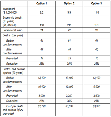
SUMMARY OF THE THREE INVESTMENT OPTIONS OF A ROAD ASSESSMENT PROGRAMME
The development of several options as in this example is fairly typical for road safety projects. This will help determine which combination of treatments will deliver the greatest benefit for the available funding. In this case, and following discussions with the project stakeholders, the options were adjusted with a lower cost option selected, and the benefits and costs recalculated. The estimated NPV of the project, using very conservative crash cost values, is US$6.1 m and the economic rate of return (ERR) is 28.8%. The ERR is well-above the Caribbean Development Bank’s cut-off rate of 12.0%
It should be emphasized that the priority listing obtained by using one of the above criteria is not ‘the perfect answer’ and other factors may come into play which affect the selection and ranking of those sites that should be treated. However, a well-grounded scheme appraisal may help to prevent emotional pressures from using up scarce resources without any other consideration. For example, if an authority is being pressured politically or otherwise to treat a site that is off this list or below the cut-off level, the table can be used to point out that resources should be focused on sites with the greatest potential benefits. This is, after all, more likely to yield the best contribution to the nation’s casualty-reduction targets.
In some cases, a site may be at a location included in a major capital works program, such as a flyover or traffic signal installation. If the implementation schedule for the program is fairly close, it may be best to ‘do nothing’ at this stage and incorporate the project into the major scheme. However, if the program is unlikely to be carried out within 2 or 3 years, short-term (perhaps lower cost) measures are probably justified.
For this and other reasons (e.g. seasonal weather preventing certain road works) that may lead to ‘slippage’ in timetables, it is always worthwhile to investigate more sites and to prepare more schemes than can be carried out in the current budget period to allow for these minor re-allocations of funds.
It is important to appreciate that the assessment of sites for treatment should be a continuous process. For example, schemes not selected for immediate implementation, either because of a low or negative NPV or because of budget constraints, should be re-evaluated at a future date if there is reason to believe the situation has changed. An increase in crashes at a site would make a scheme with a negative NPV more attractive. Other changes may also occur, such as an increase in traffic volumes, etc.
What can be stated is that investment in low-cost engineering improvements at high-risk sites can yield extremely high rates of return. For example, for general highway improvement projects, such as road re-surfacing or realignment, FYRR of 20-30% can be considered to be reasonably high, indicating projects well worth undertaking. However, low-cost improvements at high-risk sites can often produce FYRR well in excess of 100%. A significant proportion of a national road safety budget should therefore be allocated to engineering improvement projects of specific sites, along corridors or within specific areas. Such an investment is likely to pay for itself many times over within the life of the project.
Economic Appraisal Tools
A variety of tools assist with the economic appraisal process in road safety. Some examples are provided below.
SAFETY
AASHTOWare Safety is a Software as a Service (SaaS) platform designed to support transportation agencies in highway traffic safety management. The platform ingests, cleanses, and combines data for analysis. Its integrated Safety Data Warehouse stores relevant data and presents it in a user-friendly format to facilitate searching.
The Highway Safety Manual (AASHTO, 2025) outlines six steps in the Roadway Highway Safety Management Process: 1) Network Screening, 2) Diagnosis, 3) Countermeasure Selection, 4) Economic Appraisal, 5) Project Prioritization, and 6) Safety Effectiveness Evaluation. By facilitating data unification and manipulation, the Safety platform aims to provide automated insights to support agency decision-making in these areas.
COBALT (COST AND BENEFIT TO ACCIDENTS – LIGHT TOUCH)
COBALT (DfT, 2021) is an economic appraisal tool first developed in 2012 by the UK Department for Transport. It was derived from the broader transport appraisal tool, COBA (Cost Benefit Analysis tool). COBALT assesses the safety aspects of road schemes using detailed inputs for either: (a) separate road links and road junctions that would be impacted by the scheme; or (b) the equivalent links and junctions treated as single combined ‘link-junction’ pairs. The assessment is based on a comparison of crashes by severity and associated costs across an identified network in the ‘Without-Scheme’ and ‘With-Scheme’ scenarios. The comparison uses the details of link and junction characteristics, relevant accident rates and costs and forecast traffic volumes by link and junction (DfT, 2024).
ECONOMIC EVALUATION MANUAL, NEW ZEALAND
While New Zealand does not have a dedicated road safety economic appraisal tool, the Economic Evaluation Manual (EEM) (NZTA, 2013a) provides clear guidance and templates that can be used in the evaluation process. The EEM is a guidance tool outlining procedures for economic evaluations of transport investment proposals. It provides descriptions of basic concepts in economic evaluations and simple and detailed procedures for evaluations. The simple procedures are aimed at low-cost activities while the detailed procedures are for large-scale evaluations. Step-by-step methodologies for evaluating benefits and costs are also provided through downloadable spreadsheets.
There are different spreadsheets for different evaluations. The road safety promotion spreadsheet contains six procedural worksheets and four other worksheets for working notes, cost estimates and sensitivity analysis. Worksheet 1 is a summary of general project information and data used for the evaluation. Worksheet 2 is used for calculating the present value of project costs, worksheet 3 is used for calculating the social cost of crashes per person and worksheet 4 is used for calculating the present value of project benefits. Worksheet 5 is used to calculate the BCR per head. The cover worksheet is a summary of all the information and calculations in the spreadsheet. For each of the steps, there is guidance offered on the necessary information and input data.
OTHER TOOLS
European guidance on economic appraisals and prioritisation of road safety countermeasures is also available to practitioners. Examples of this include the European Road Safety Observatory (ERSO), and the EU projects HEATCO (Harmonised European Approaches for Transport Costing and Project Assessment) and ROSEBUD (Road Safety and Environmental Benefit-Cost and Cost-Effectiveness Analysis for Use in Decision-Making).
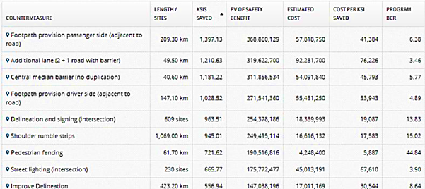
The process applied by iRAP (see Road Assessment for Safety Infrastructure in Section 10.4 Proactive Identification) not only identifies problems and effective interventions, it also produces detailed business plans, including the cost-effectiveness of the interventions identified. An example from the Ukraine of one such investment plan is provided in Figure 11.9.