12.4 Evaluating Road Safety Infrastructure Interventions

Effective decisions regarding the use of road safety infrastructure interventions can only be made with adequate knowledge regarding its effectiveness. The key measure that is used for this assessment is the expected reduction in crashes, expressed as a crash modification factor (CMF) for the intervention. This indicates the degree to which the intervention is expected to reduce crashes. CMFs are also described in detail in Effective Safe System Interventions in Section 11.3. Intervention Options and Selection. CMFs help policy- makers in the decision-making process, and the results from previous studies are typically used to provide a realistic estimate of the expected effect (SafetyCube and CMF Clearinghouse). However, there are many gaps in knowledge regarding the effectiveness of interventions.

An international collaboration on effective evaluation for road safety infrastructure interventions has been completed in 2012 by the OECD (Sharing Road Safety - ITF, 2012) which provided the following key messages:

• Road safety policy is increasingly dependent on robust indicators on the effectiveness of interventions. This information is required to justify expenditure, and also to argue for support of interventions that may not always be popular. CMFs are fundamental in this context.
• Lack of reliable knowledge of the effectiveness of certain road safety infrastructure is a key barrier to the adoption of potentially life-saving interventions.
• We are currently at a turning point, as there is the prospect of rapid advances and major cost savings through the international transfer of results on treatment effectiveness (e.g. via CMFs).
• Transferability of CMFs relies on analysing the extent to which a CMF is dependent on the circumstances/context/environment in which it was developed (also see Chapter 11 Intervention Selection and Prioritization on this issue of context).
• Variability in CMF research results is a major barrier to transferability between countries, but this can be addressed by using standard approaches to evaluation, including appropriate methodologies and reporting of the circumstances under which the intervention was used (guidelines for developing and applying CMFs were published in the NCHRP research report 991 – National Academies, 2022).
• An additional difficulty is related to the evaluation of CMFs when implementing several interventions combined together.

Some of the key recommendations from this work were that:

• Road safety policies should undergo performance and efficiency evaluation. This work cannot be undertaken without CMFs.
• Research to develop CMFs should follow the guidance presented in the OECD report (ITF, 2012) report and provide information on essential reporting elements.
• Coordination of research across countries on top priority countermeasures should be considered within an international group.
• A trans-national database is needed for CMFs to help share information.
• A concerted effort should be made to publicise the benefits of decision-making based on CMFs.

The ultimate measure of the success of a road safety policy or intervention is the effect that it has had on crash reduction, particularly the reduction in fatal and serious injuries. Unfortunately, difficulty arises in considering crashes on their own, as it may be necessary to wait several years after the countermeasure or package of measures has been introduced to be able to validate the changes in crash statistics. Given an indication of effectiveness is often required in a shorter timeframe, particularly to determine that nothing has gone wrong, more immediate feedback may be required. Proxy measures for safety might be useful to monitor the effectiveness of schemes (see also Section 5.2. Identifying Data Requirements) for the link between intermediate and final outcome measures. These proxy measures are usually observational-type measurements. It is often recommended to conduct an evaluation in two stages: a short-term phase (e.g. 6 months) and a longer-term phase (e.g. 3 to 5 years).

Observations

Where practical, the treated site, route or area should be observed immediately after completion of the construction work, with regular visits made in the following days, weeks or months after completion until the team is satisfied that the scheme is operating as expected.

It is recommended that any earlier behavioural measurements made at the investigation stage be repeated later (e.g. traffic conflict counts, speed measurements, etc.), as this will help determine/support the need for any further changes, or may in fact prove the success of the intervention. This behavioural study is also required because some features of an intervention may, for instance, produce an unforeseen reaction in road users and subsequently create a potentially hazardous situation. Monitoring and analysis should highlight this problem at an early stage so that appropriate action can be taken quickly to remove this hazard.

At best, it may be possible to alleviate this hazard easily, e.g. by realigning the kerb lines to prevent a hazardous manoeuvre. At worst, it could lead to the complete withdrawal of a scheme and the need to reassess alternative schemes.

Some of the issues that may be relevant to assess include:

• Speeds.
• Traffic conflict studies.
• Traffic volumes.
• Travel time/delay.
• Compliance with traffic control devices.
• Skid resistance.
• Sight distance.
• Vulnerable road user safety (nature and importance of users’ movements).

It would be impractical to carry out detailed behavioural studies for all minor alterations, but such studies may be particularly important for expensive schemes such as area-wide or mass action treatments.

Specific studies on pedestrian movements should also be undertaken if the collision records show that a high proportion of crashes that involve pedestrians. Similarly, a high incidence of skidding under wet road conditions may indicate the need for specific studies on skid resistance (also associated at times with the use of limestone aggregate). In developing countries where road user behaviour is often poor, studies on driver behaviour at signals, pedestrian crossings, and uncontrolled intersections may also be worthwhile.

It may be preferable to allow the scheme to operate for about two months before conducting a behavioural ‘after’ study. This should serve as a ‘settling-in’ period, during which regular users get used to a new road feature and any learning effects have largely disappeared. The evaluation should verify the impacts in terms of safety for all users. The overall effects of a project should be understood as a whole. For example, the implementation of a bike lane can be dangerous if used by motorcyclists.

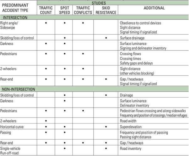
The nature of the identified crash problems at the site should guide the choice of studies to be conducted. Table 12.1 provides indications in this respect.

TABLE 12.1: STUDIES THAT MAY BE APPROPRIATE FOR PARTICULAR CRASH PROBLEMS

TRAFFIC SPEED

Speeding is frequently reported as being a major contributing factor in crashes, and there can be no disputing the fact that speeding reduces safety margins and the likelihood of escaping injury. If speed reduction is one of the objectives of the scheme, then speeds should obviously be monitored. Similar and appropriate locations should be carefully chosen for the before and after studies, preferably using automatic equipment.

The Technical study - Spot Speed describes how to measure speeds.

A Student t-Test can be used to determine whether any changes in the measured mean speeds between two measurement periods are statistically significant or, indeed, whether there is a significant difference between the speeds of different vehicle types (e.g. passenger cars and trucks). Changes in the actual distribution of speeds following introduction of a speed-reducing measure can be tested with the Kolmogorov-Smirnov test.

CALCULATOR: SPOT SPEED STUDY

CALCULATOR: DISTRIBUTION TEST

TRAFFIC CONFLICTS

The collection of accurate traffic data is important when comparing crash sites. The traffic data needs to be compatible with the crash data (e.g. for the same period) and in sufficient detail to be appropriate for the particular evaluation. If a countermeasure is expected to affect manoeuvres at an intersection or drivers’ choice of route in any other way, then traffic flow data should be collected throughout the local network before and after introducing the measure.

The number of vehicles and pedestrians passing through a site will provide useful information on the exposure to risk of the various road user groups. If, for example, significant proportions of cyclists and corresponding crash types have prompted the introduction of segregated cycle lanes, it will be important to monitor how well these are being used and whether they have attracted new cycle traffic.

The Technical study - Traffic Count describes how to conduct this study.

TRAVEL TIMES

In some cases, monitoring may require an estimate of changes in travel time for residents and through traffic by carrying out ‘origin and destination’ travel time studies. This will be important where traffic severance forms part of the scheme, and traffic is being re-routed. In economic evaluations (Chapter 7), if the extra time lost due to re-routing is likely to be significant, then value-of-time considerations should be taken into account (as a disbenefit).

The Technical study – Travel Time and Delay describes how to conduct this type of analysis.

PUBLIC PERCEPTION

Often one of the main reasons for implementing an area-wide scheme is that residents may have campaigned strongly for something to be done. One of the most important parts of an area-wide scheme, therefore, is public consultation. Thus, one factor to monitor is how the residents and other road users feel about the safety elements of the scheme.

Ideally, public attitudes should be assessed before a scheme is implemented by posting questionnaires on social media or sending them by email conducting interviews with residents and interviewing road users in the treatment area. The public should, of course, be informed about the details of a proposed scheme, as well as its necessity and suitability, before its implementation. A similar survey should then be conducted several months after the scheme has been installed to monitor general and specific satisfaction (or dissatisfaction).

EFFECTS ON ADJACENT AREAS

Some schemes can affect adjacent areas, possibly leading to an increase in traffic speeds, volumes and crashes. Thus, it is important to monitor these factors carefully in all relevant areas adjacent to the road(s) where the scheme was introduced.

The following six case study from Malaysia, Puerto Rico, Portugal, Slovakia and Italy provides a number of excellent evaluations on the safety effects of various treatment.

Crash-based Evaluation

The most important form of evaluation of any safety measure is determining its effect on crashes, and whether the intervention has reduced the number of crashes (particularly fatal and serious injury ones) by the expected amount. Evaluation involves the analysis of crash data by comparing the safety performance before a change was made to the safety performance afterwards. This often involves statistical analysis.

To be reasonably sure that the random nature of crashes has been taken into account, it will normally be necessary to wait for several years for sufficient and statistically significant results to be available to conduct reliable before/after crash analyses. It is therefore essential to complement the use of such before/after crash analyses with appropriate technical studies and site observations (shorter-term monitoring methods) that provide useful information on a treatment effectiveness soon after its implementation (spot speed study, traffic conflict study, etc.).

Apart from the time-scale issue, there are other factors that complicate the (apparently straightforward) process of assessing the effectiveness of crash changes at treated sites, routes or areas. The main ones to consider are:

• Regression to the mean.
• Changes at the site that are not related to the intervention (including general changes to crash trends, changes in traffic volume, etc.).
• Crash migration.

Each of these is discussed after the evaluation methods.

EVALUATION METHODS

In evaluating a particular treatment, the answers to the following questions will usually be required:

• has the treatment been effective?
• if so, how effective has it been?

The rare and random nature of road crashes can lead to fairly large fluctuations in frequencies at a site from year to year, even though there has been no change in the underlying safety level. This extra variability makes the effect of the treatment more difficult to detect, but a test of statistical significance can be used to determine whether the observed change in crash frequency is likely to have occurred by chance or not.

There are several key documents that provide detailed accounts of evaluation methods for road safety infrastructure. These include:

• The Highway Safety Manual (AASHTO, 2025).
• An Introductory Guide for Evaluating Effectiveness of Road Safety Treatments (Austroads, 2012).
• Guide to Developing Quality Crash Modification Factors (Gross et al., 2010).
• Guide for Road Safety Interventions: Evidence on What Works and What Does Not Work (Turner et al., 2020).
• Guidelines for the Development and Application of Crash Modification Factors (National Academies, 2022).

One or more of these documents should be consulted for a full account of how to conduct a road safety evaluation.

When evaluating changes in crashes, other factors not affected by the treatment, and which might also influence that measure, have to be taken into account. Examples include a change in the speed limit on roads that include the site; national or local road safety campaigns; traffic management schemes that might affect volumes of traffic: e.g. closure of an intersection near the site, producing a marked change in traffic patterns.

These features can be taken into account by using control site data, but in order for this to be valid, it is important that these other sites experience exactly the same changes as the site under evaluation.

The ‘gold standard’ in evaluation methodology is a ‘controlled experiment’ or Randomised Control Trial (RCT). As indicated earlier, this approach is very rare in evaluation of infrastructure interventions. This is mainly due to concerns with leaving high risk sites untreated, but is also due to issues such as lack of knowledge regarding this approach. By randomly allocating sites to a treatment or control group, any biases which arise from treating sites with the worst crash history should be eliminated. External factors which come into play as the evaluation proceeds (such as unforeseen enforcement programmes in the area of the trials) are also catered for, as the external factors can be assumed to affect the treatment and control sites equally. The difference between the treatment and control sites in the after period is a true reflection of the influence of the treatment.

The currently recommended approach for evaluation of infrastructure interventions is the Empirical Bayes (or EB) method (for more details see Empirical Bayesian Methods in Section 10.3 Crash-based Identification (‘Reactive’ Approaches)). Hauer (1997) explains this procedure in its simplest form, which is recommended reading for those wishing to understand the logic behind this approach as it applies to road safety. The approach uses the concept of an ‘expected’ number of crashes, or the long-term average, calculated over as long a period as is considered useful. The second concept is the ‘reference population’, or a set of similar sites or routes for which date is available (e.g. all intersections of a certain type in a network). The reference population acts like a comparison group. In the classical version of EB, the number of crashes which would be expected at a treatment site if no intervention had taken place is estimated and compared with the number of crashes that actually occurred. The comparison of the actual number of crashes with the expected number of crashes indicates the extent of the CMF.

Control Sites

Another method commonly applied for the evaluation of infrastructure safety is the before-and-after study utilising a comparison group. Even though this approach does not fully address the issue of regression to the mean, it does limit the impact of external factors. The approach compares the outcomes at the treatment sites with the outcomes at a set of comparison sites (sometimes termed ‘control sites’), which have similar characteristics to the treatment sites in all important aspects, except that the treatment is not installed. This approach assumes that external factors act on both the treatment sites and the comparison sites in an identical way, and so can be measured and allowed for. Since the treatment sites and the comparison sites are subject to the same sets of external variables, any difference in safety outcomes must be due to the treatment.

Changes related to external factors may be compensated for by comparing the site under study, for the same before and after periods, with ‘control sites’ that have not been treated. Control data can be collected either by matched pairs or area controls.

Although the matched pair is the best statistical method, in practice it may be difficult to find other sites with similar safety problems that will be left untreated purely for the sake of statistical tests. Area controls comprising a large number of sites are, therefore, much more frequently used.

When choosing sites for control groups:

• they should be as similar as possible to treated sites.
• they should not be affected by the treatment.
• the control area should be as large as is reasonable: as a guide, try to find a similar area or group of roads that have more than 10 times the number of accidents than the treated sites have.

For example, if the traffic signals at a site are to be modified, the engineer could choose all the other signalized intersections in town as the control group. If, however, there are only two other signalized intersections, and these had lower flows and much fewer crashes than others uncontrolled intersections, it would be better to use, for example, all signalized intersections in the state/county.

The most basic form of evaluation (and one that has often been applied) is to simply compare crashes in the period before an intervention is installed with the crashes after (termed a simple or naïve before-and-after study – i.e. without a comparison group). This approach is not recommended, as it does not adequately account for regression to the mean or external variables.

Cross-sectional studies have also been used to try and identify the effects of safety interventions. These studies compare safety performance of sites with a particular safety feature (or features) with sites that do not have the same feature. It is assumed that the difference in safety performance is due to this feature. There are many issues with using this approach (particularly differences between sites other than the feature of interest, and higher crash rates that may have led to the installation of the feature in the first place), therefore it should not be used for this type of evaluation (however, if it is used, the limitations should be well-understood and documented).

The main problem with using crash data for evaluation (even assuming high recording accuracy) is distinguishing between changes due to the treatment and changes due to other sources. Even if the selected sites are good comparison groups that take into account the environmental influences, there are other confounding factors that need to be considered.

There are a number of points to take into account when choosing time periods used to compare crashes occurring before and after treatment. These include:

• The construction period should be omitted from the study. If this period was not recorded precisely, a longer period containing the installation period should be excluded.
• The before period should be long enough to provide a good statistical estimate of the true safety level (to eliminate random fluctuations as much as possible). It should not, however, include periods during which the site had different characteristics. As a general rule, three to five years is widely regarded as a reasonable period.
• The same rule applies to the after period, which should be at least three years. However, results are often required much sooner than this. A one-year after period can initially be used if there is no reason why this should bias the result (as long as the same period is used at the comparison sites). However, sensitivity is lost, and the estimate of the intervention’s success should be updated later when more data becomes available.

Clearly, this section of the manual cannot deal with the complex principles underlying the various statistical tests that can be used in crash investigations and for this the reader should refer to standard manuals on the subject. However it does cover, albeit briefly, various statistical tests that can be used to answer the key questions posed at the beginning of this section, i.e. has the treatment been effective and, if so, how effective has it been?

For this purpose, it is sufficient to assume that the before and after accidents are drawn from a normal (or Gaussian) distribution. In other words, the distribution of accidents in a sample is symmetrically drawn from either side of a mean value.

This means that we can use the ‘Chi-square’ test to answer the first question as to whether the remedial action has been effective, i.e. whether the collision changes at the site are statistically significant. If the same type of remedial treatment has been carried out at many sites, an additional calculation is required in order to determine the overall effect.

Appendix 12.1 presents a brief description of some of the main statistical tests associated with transport project evaluation. Table 12.2 provides a list of these tests and their condition of use.

As identified throughout this chapter, there are a number of documents that provide a detailed guide to evaluating intervention effectiveness. There are also various tools to help with this task. An estimate of the effectiveness of treatments in terms of percentage of potential casualty reduction is also provided by the iRAP Toolkit.

BOX 12.1 SAFETY ANALYST COUNTERMEASURE EVALUATION TOOL

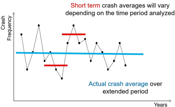
Regression to the mean

This effect complicates evaluations at high-crash locations. Crash locations for treatment are typically chosen because they were the scene of numerous crashes. In some cases, the high crash numbers may be the result of just one particularly bad year, and this may have happened purely by chance.

Crash numbers at such sites will tend to fall in the next year even if no intervention is applied. Even if a three-year period is used, crash occurrence may be due to random fluctuations, and in subsequent years these sites will experience lower numbers. This is known as regression to the mean. According to different international studies (an example is in Box12.1), it is believed that the regression to the mean effect can overstate the effectiveness of a treatment by 5% to 30%. Figure 12.4 shows a graphical representation of regression to the mean.

BOX 12. 2 EXAMPLE OF REGRESSION TO THE MEAN

The most robust way of accounting for both the regression to the mean effect and changes in the environment may be through the use of control sites that have been chosen in exactly the same way as the treated sites and have been identified as having similar problems, but have been untreated. The choice as to whether a site is treated or is untreated is based on a random allocation. This type of controlled experiment (or Randomised Control Trial) is rare in road safety infrastructure projects as it is difficult to justify not treating a site that has been identified as high risk.

In recent years, the Empirical Bayes approach (for more details see Empirical Bayesian Methods in Section 10.3 Crash-based Identification (‘Reactive’ Approaches)) has emerged as an effective way of minimising the impact of regression to the mean. Although the Empirical Bayes approach is recognised as good practice in road safety evaluation, not all countries (especially those in LMICs) will have experience in using this technique.

If not using this recommended approach, at the very least, a before-and-after analysis using comparison sites should be undertaken, with at least three (but preferably five) years of data collected for the before period. This is because the regression to the mean effect does tend to diminish if considered over longer periods of time. For example, in a study conducted in two counties in the UK, Abbess et al. (1981) calculated that regression to the mean had the following effects:

• When a one-year period was used, the effect of regression to the mean was estimated to be between 15-26%.
• For two years, the estimate was 7-15%.
• For three years, the estimate was 5-11%.

Where the Empirical Bayes approach has not been used, the above allowances could be made when calculating the reduction in crashes produced by the countermeasures.

A method described by Abbess et al. (1981) is outlined in Appendix 12.1. The ‘regression-to-mean’ calculator is based on this method.

CALCULATOR: REGRESSION TO THE MEAN

CHANGES IN GENERAL CRASH TRENDS, INCLUDING TRAFFIC FLOW

When evaluating changes in crashes (or for most of the monitoring measures described in Observations), other factors not affected by the treatment might still influence that measure, and therefore will have to be taken into account. Examples include a change in the speed limit on roads that include the treated crash site, national or local road safety campaigns, or traffic management schemes that might affect traffic volume (e.g. closure of an intersection near the site, producing a marked change in traffic patterns). Changes related to external factors may be compensated for by comparing the site under study, for the same before and after periods, with comparison sites (or ‘control’ sites) that have not been treated. In order for this data to be valid, it is important that these other sites experience exactly the same changes as the site under evaluation.

Comparison data can be collected either by matched pairs or area controls. A matched pair control site involves finding a site that is geographically close to the treated site (but not close enough to be affected by any traffic diversion) and has similar general characteristics. This is so that the control site will be subject to the same local variations that might affect safety (e.g. weather, traffic flows, safety campaigns, etc.).

In practice it may be difficult to find other sites with similar safety problems that will be untreated purely for the sake of statistical analysis. Area comparisons comprising a large number of sites are, therefore, frequently used.

Comparison group sites should be as similar as possible to the treated sites, and they should not be affected by the treatment.

CRASH MIGRATION

There is still some controversy over whether or not the ‘crash migration’ effect exists. It has been found that crashes tend to increase at sites adjoining a successfully treated site, producing an apparent crash transfer or ‘migration’. Why this effect occurs is unclear, but one hypothesis is that drivers are ‘compensating’ for the improved safety at treated sites by being less cautious elsewhere, especially those who know the area well and are familiar with it.

Obviously, to detect such an occurrence, the crash frequencies in the surrounding area of the treated sites before and after treatment need to be compared with a suitable comparison group. In other words, the area of an evaluation study needs to be expanded to include routes that may be impacted by the project, and comparison sites must be identified that have not been affected.

However, there are no established techniques yet available to estimate such an effect for a particular site. The first reported occurrence of this feature (Boyle & Wright, 1984) found an overall crash increase in the surrounding areas of about 9%, and a later study (Persaud, 1987) of a larger number of sites estimated the increase to be 0.2 crashes per site per year.

A study by Austroads (2010) identified the effects that certain interventions have on the redistribution of traffic, and suggest that this may be a cause of migration. If traffic is reduced at the treated location, it is likely that it will be increased at a nearby location (this is likely in all situations, except the rare circumstance where trip numbers are reduced). It is suggested that this redistribution is more likely for certain types of treatments. For these interventions, evaluation of the effects should include a broader geographic area to capture locations where exposure (and therefore risk) may be increased. Interventions identified as potentially causing such an effect included:

• Turn controls or bans.
• Major changes to a route, such as parking changes.
• Bridge closure.
• Localised speed limit changes.
• Intersection changes, e.g. signalisation, turn phase timing change, turning lanes.
• Traffic calming.
• Lane additions.
• Addition of overtaking lanes.
• Pedestrian treatments at intersections and at mid-block locations.
• Railway crossing control.
• Mid-block turning provision.

GRAPHICAL ANALYSIS

A simple visual method that has been used in some countries (e.g. Radin Umar et al., 1995) is to monitor the trend in crashes over time. In this method, the cumulative crash numbers (and types) are plotted together with their cumulative mean (see definitions below).

However, it should be noted that this is more useful for mass-action plans and not really suitable for single sites (due to the lower numbers of crashes involved).

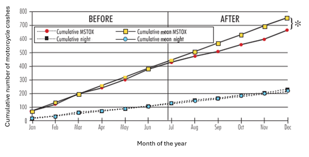
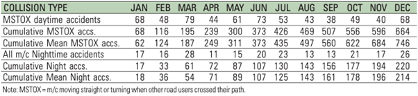
An example is shown in Figure 12.4, where the graph illustrates that a Malaysian motorcycle daytime running headlight campaign was apparently effective in reducing collisions related to daytime conspicuity (MSTOX = motorcycles moving straight or turning when other road users cross their path) while, as might be expected, having no effect on nighttime crashes.

The table in Figure 12.4 shows the monthly cumulative frequency of related crashes in the second row, which totals the actual number of crashes six months before and after the measure (end of June). The cumulative mean (third row of the table) is obtained by simply calculating the average monthly crash frequency over the before period (in this case 6 months) as the first month and then adding this figure onto each subsequent month. This is the number of crashes that one would have expected, had the measure not been taken. Lines 5 and 6 of this table show an equivalent number for night crashes. In this case, the cumulative means are:

For MSTOX crashes: (68 + 48 + 79 + 44 + 61 + 73) / 6 = 62

For nighttime crashes: (17 + 16 + 28 + 11 + 15 + 20) / 6 = 18

It can be seen that during the after period (July to December), there is an increasing gap between the observed number of daytime crashes (second row) and the expected number of crashes (third row). Since the expected number is larger than the observed number, the measure is seen to have had a positive effect. The (✽) sign in Figure 12.5 represents the effect of the measure. In comparison, the observed and expected number of night crashes remain quite similar in the after period.

However, as already stated, to be sure that the random nature of collisions has been taken into account, a much longer waiting period is normally required (usually three years) for a statistically valid result to be available. For more immediate feedback, other behavioural data, as mentioned in the previous sections, should be collected to give indications that a scheme is working as intended.

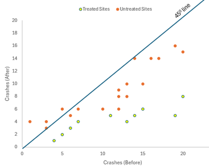
Where control sites (or similar untreated sites) have been selected, another simple exploratory method for displaying the change in collisions at several treated sites has been described by Ogden (1996). For each site in both the control and treated groups, collisions in the before period and after period (of the same length) are plotted as shown in Figure 12.5 If there was no change in the number of crashes between the two periods, then all the points would lie around a 45-degree line. The extent to which there is a change in the after period is indicated by the departure from the 45° line.

If, as in Figure 12.6, the treated sites are trending markedly below the untreated sites, then it is suggested that the treatment is having a positive effect.

ECONOMIC EVALUATION

As discussed in Chapter 11 Intervention Selection and Prioritisation, for every scheme the evaluation should include an indication of the benefits actually achieved in relation to cost. Even if the scheme has been designed to tackle a very specific target group of crashes, it is normal practice to include all collisions at the site in a full evaluation – just in case the measure has had an unforeseen effect on other crash types.

Appendix 12.1 describes how the collision impact of a specific road improvement can best be estimated. Suppose that the estimated reduction was 68% (this is the result obtained in the example of Appendix 12.1 – k-test). If the site was one of the worst in the district, then we ought to make some allowance for the regression-to-mean effect (e.g. Table 12.2). Let us assume this amounts to as much as 11%, such that our best estimate of the true reduction in crashes is 57% (68% - 11%).

Since the original number of crashes in this example was 20, 11.4 crashes have been saved over the study period (or 3.8 per year).

It should be noted that only injury crashes have been considered here but if there are a number of damage-only occurring that are reliably reported, then these should also be included in the costing. However, it must be stressed that in most countries of the world, damage-only crashes are frequently not reported to the police and are thus a much more unreliable measure.

Based on an average injury-crash cost of $79,330 that has been used in the examples of the previous chapter, this collision saving amounts to $301,454 per year. This figure is then compared to treatment costs, i.e. $298,000. Assuming traffic delays due to the treatment are negligible, the First Year Rate of Return (FYRR) equals:

FFYRR = 301,454/298,000 x 100 = 101.2%

The above FYRR figure should be rounded down to 101% to give an indication of the possible effect of using this treatment in the future.

Other economic criteria that have been described in the previous chapter could also be used. For example, the calculation of the Net Present Value (NPV) figures would be particularly advisable if, over future years, there are known to be inevitable new maintenance costs associated with the installed measure.

It is only by evaluating and recording results in this way that a database of implemented remedial measures and their effectiveness can be assimilated for use by road authorities throughout the country.

OVERALL EFFECTIVENESS AND FUTURE STRATEGY

This chapter has set out methods that can be used for evaluating the effects of particular schemes and strategies. One way of publicising these results is for the road safety unit within a highway authority to produce a regular strategy document that outlines its main road safety achievements as well as the projected work.

A summary of this strategy document should be included in the official road safety action plan of a country. This plan also includes, as background information, aggregate crash statistics by state, district, or municipality, broken down into various categories, such as road user class, road class, etc. These aggregate figures can be useful not only to indicate general priorities, but also to evaluate the effects of wide-scale safety campaigns, as well as legislative and/or enforcement changes.

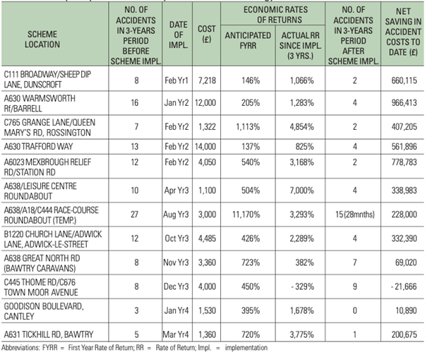
However, as schemes are usually localised, their effects are often difficult to detect among much larger collision totals. Hence, the strategy document should probably include a summary listing of the effectiveness of all low-cost schemes (e.g. Table 12.4). This is more informative than a single overall figure as it displays the range of safety efforts taking place and the relative success of the various actions. The official publication of past achievements and future plans has been found useful not only in making the highway authority’s road safety team accountable, but also in helping the team focus its efforts on a long-term casualty-reduction target. The document also provides valuable information to other workers, giving real evidence of the extent to which schemes are successful.

TABLE 12.4: EXAMPLE REPORT ON LOCAL SAFETY SCHEME EVALUATION FROM A STRATEGY DOCUMENT