10.3 CRASH-BASED IDENTIFICATION (‘REACTIVE’ APPROACHES)

This section focuses on crash-based identification of high-risk locations, a process that is known as crash investigation, or the treatment of ‘high-risk location’. The term ‘sites with potential for safety improvement’ is also used, as the approach involves selecting locations that have high potential for reductions in crashes through the introduction of targeted safety improvements. The approach relies on crash analyses to first identify safety problems before a solution is sought. These are often called ‘reactive’ methods because a response is only initiated after crashes have occurred. A fuller account of this approach is provided in the PIARC document Road Accident Investigation Guidelines for Road Engineers (PIARC, 2013).

As indicated above and in Section 10.4 Proactive Identification, reliance solely on crash data can produce situations where only a small proportion of crashes can potentially be addressed. For this reason, it is recommended that a combination of crash data and other sources of information be used to assess and treat risk.

Reactive approaches typically include the following steps:

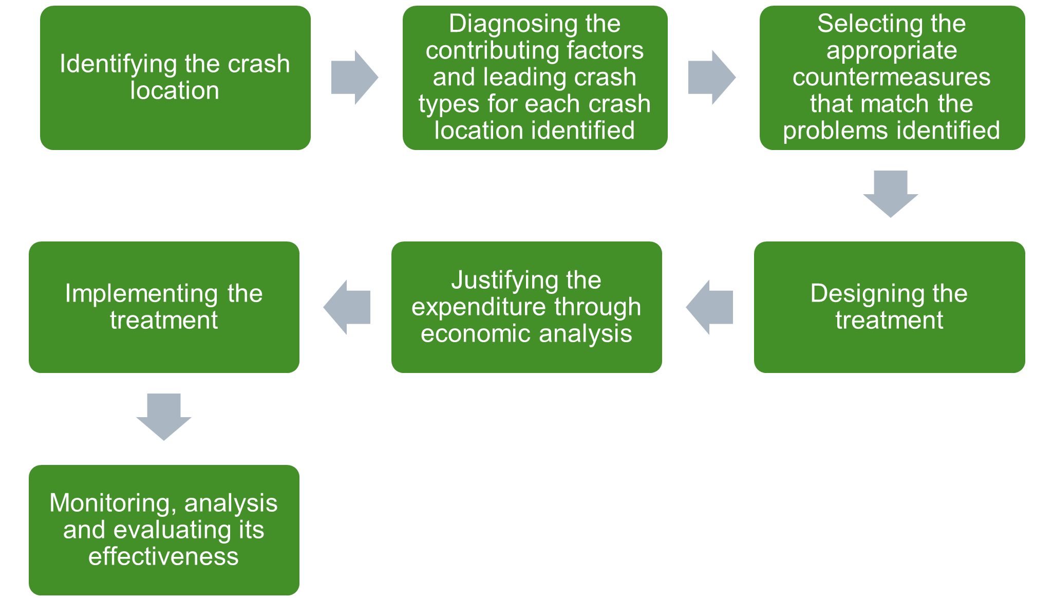
This chapter focuses on the first two points – identification and diagnosis. Consideration will also be given to how crash data is used and its limitations. The other steps will be covered in Chapter 11. Intervention Selection and Prioritisation and Chapter 12. Monitoring, Analysis and Evaluation of Road Safety Interventions. A reliable crash database is a key tool in this process of identifying and analysing crash locations (see Hospital Data in Section 5.3 Establishing and Maintaining Crash Data Systems). Other tools also exist, for example the Network Screening and Safety Analysis in AASHTOWare Safety (see Box 9.5 in Section 9.4 Management Tools).

USING CRASH DATA

In order to treat the occurrence of crashes, crash data is needed to provide necessary information to road authorities. Further information on the collection and use of crash data can be found in Chapter 5. Effective Management and Use of Safety Data. Issues relating to the need for good quality data are also discussed in that chapter. To ensure adequate data quality, the data should fulfil the following basic requirements (PIARC, 2013):

• Accuracy (to exactly describe the individual parameters).
• Complexity (to include all features within the given system).
• Availability (to be accessible to all users).
• Uniformity (to apply standard definitions).

The primary data source for crash reduction initiatives, especially those undertaken by road engineers, is typically police crash reports. This data should provide crucial information, which at a minimum should include the crash severity and the number of each injury severity type (i.e. fatal, serious, minor, etc.).

A (non-exhaustive) list of other important information to collect includes (PIARC, 2013):

• Crash identification number.
• Information about the crash site (e.g. an accurate location).
• The occurrence of events that resulted in the crash (e.g. the crash type).
• Information on those involved (gender, age, road user type, whether alcohol was involved, use of seatbelts, etc.).
• Weather and lighting conditions.
• Vehicles involved.
• Time of day, day of week, and date.

Crash type is of particular importance, as it provides the basis for some crash location selection criteria (as discussed in the following section). Normally, crash types are divided into groups of crashes with common attributes, such as all crashes involving vehicles colliding head-on, or all crashes involving pedestrians.

IDENTIFYING CRASH LOCATION

It is important to be able to identify the location where a crash occurs. A crash location can be an individual site (such as an intersection or bend in the road), a segment of road, an area of the road network (such as an entire corridor), or a collection of locations across the network (road system wide) that display the same crash characteristics. In order to identify crash locations, access to a comprehensive database is required to provide sufficient information about the exact locations and circumstances of crashes that have occurred. Once all crash sites have been located, there needs to be selection criteria so that only worthy sites are selected for further analysis and treatment.

The following sections provide an overview of the approaches that can be used in identifying crash locations. Detailed guidance on the identification of high-risk locations has been developed in many countries. In addition to the PIARC (2013) manual, further information can be gathered from many sources, including AASHTO (2025), Austroads (2021), and RoSPA (2007). The African Development Bank (2014a) has released guidance that is specifically intended for use in LMICs.

DEFINING LOCATIONS

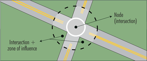
High risk locations are often located at nodes of the road network, i.e. at crossing points between two or more roads (conventional intersections, roundabouts or interchanges), or walking, biking, or trail crossings. Crash concentrations are also often found on short links such as sharp curves or steep hills.

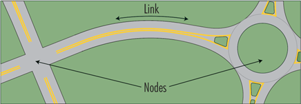
Since crash densities differ at nodes and along links, these two types of sites should be distinguished during the identification process. Otherwise, some links could be identified as deviant simply because they contain one or more nodes.

It is important to consider what the boundaries of a crash location are. There needs to be a defined cut-off point, such as between crashes that occur at or because of an intersection and crashes that are considered ‘mid-block’ (i.e. on a link between two intersections). It may be necessary to look beyond these defined boundaries when analysing crash data. For example, crashes within 10 metres on the approach roads to an intersection may be considered as located at the intersection (‘zone of influence’ of an intersection); however, it may be of value to look beyond this boundary for other crashes that may be related to an intersection (e.g. 100 metres). To avoid biases at the identification stage, the same zone of influence should be used for all similar nodes in similar road environments.

The unit length for a road link that is used at the identification stage has an impact on the choice of sites that are detected. Overly long links can prevent the detection of local crash concentrations, which will be diluted in the surroundings, and on the other hand, overly short links will have either 0 or 1 crash, in which case the information is of little use. Link lengths ranging from 500 m to 1,000 m are usually adequate for identification purposes.

Either fixed sections or mobile sections (‘sliding windows’) can be used to identify hazardous links. The use of fixed sections is simple: a fixed origin is determined and the road is subdivided from this point into successive sections of equal length. However, it can prevent the detection of crash concentrations located at the boundary of two adjacent sections. The use of mobile sections that shift a constant section length, e.g. 1 km, along the road by means of a short increment, e.g. 100 m, eliminates this problem. Detection criteria should be set to identify the high-risk locations. Many European countries use the sliding window in their national network analysis methodology, i.e. Austria (Nowotny, 2019; ASFINAG, 2011), Belgium - Flanders region (Geurts and Wets, 2003), Croatia (Saric et al., 2016), Denmark (Danish Road Directorate, 2014), Hungary (Borsos et al., 2016), and Lithuania (Lietuvos Respublikos Susisiekimo Ministro, 2011).

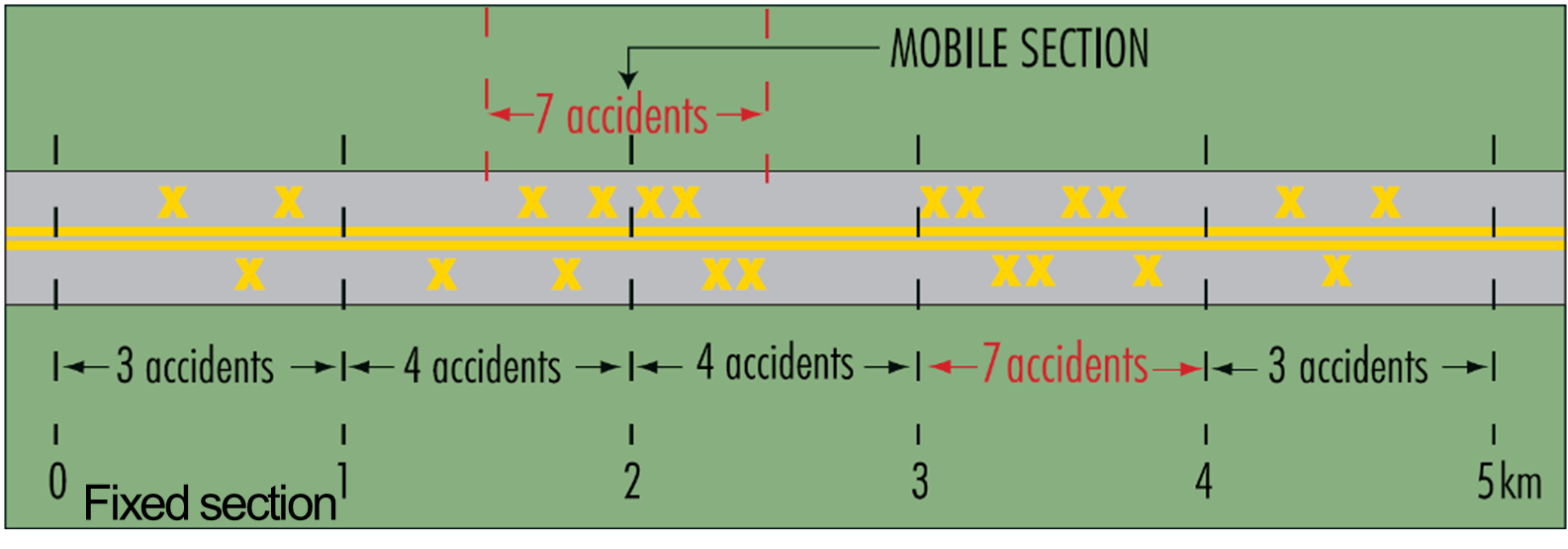
Figure 10.8 illustrates the usefulness of this method. Assuming a detection threshold of 7 crashes/km, the crash concentration located between kilometres 1.5 and 2.5 would not be detected with a fixed section, but it would be with a mobile section.

Computerized databases now simplify the use of mobile sections and increase the possibilities. For example, the beginning of each constant section could coincide with the exact location of each crash in the database, which increases accuracy while avoiding useless computations. Hauer (2004) instead recommends using not only variable starting points but also sections of variable lengths.

The crash location is also generally identified as the point at which an impact occurred. However, this may only be the end point of a sequence of events. Factors relating to the cause of the crash may have started earlier on the roadway.

Crash locations can sometimes be poorly or inaccurately defined, and it is important to consider this when comparing crash sites. There are a number of different methods used to determine the location of a crash. In built-up areas, the common practice is to measure the distance from the nearest intersection, junction or landmark using some distance measuring device. However, in rural areas and in some countries in general, names may not exist for all roads, and junctions may be few and far between. Other common systems are the Linear Referencing System and Link-Node System. These two rely on road names or reliable kilometre post markers along roads. In many countries hectometre points (or milepost) on road are a part of infrastructure for a very long time. Those signs are helping to identify number and kilometre (or milepost) of the road. Now more and more common is to use Global Positioning Systems (GPS). This is the recommended system for data accuracy. Gathered in this way latitude and longitude coordinates may show us the exact location more precisely. For roads where the infrastructure does not contain kilometre and/or hectometre (milepost) signs it is important to consider if it is more effective to invest directly into a GPS solution because of its advantages in locating crashes. See Chapter 5. Effective Management and Use of Safety Data and WHO (2010) for more detail on using reliable and accurate data to identify high risk locations.

Over time, especially in HICs, there has been a movement to the assessment of more extensive areas, including route-based approaches. The term ‘Network Safety Management’ is used in Europe to encompass an approach that assesses extended routes, typically between 2 and 10 km (Schermers et al., 2011). These segments have higher than expected numbers and severity of crashes when compared to other similar segments. Various tools have been developed to help with this process, and some of the key approaches are discussed below.

DECIDING ON A TIME PERIOD

Typically, a three- to five-year period is selected to provide a large enough sample of data for statistical reasons (regression to the mean), whilst minimising the chance of changes to the road network. In some LMICs, high risk locations and crash patterns within a location may start to form after just one to two years. Once a strong pattern has been established, especially where fatal and serious injury crashes are occurring, it is more important that treatments are implemented earlier rather than waiting up to three or even five years for more data. When selecting the time period, it is important to use whole years to avoid cyclic or seasonal variations in the crash and traffic data. It is also important to be aware of any changes in database definitions that may have occurred in that time or the presence of periods to be excluded due to exceptional events that have caused significant changes in the traffic data and thus crash data (e.g. wars, epidemics such as Covid, etc.).

CRITERIA FOR SELECTING LOCATIONS TO INVESTIGATE FOR TREATMENT

There is generally not enough funding to treat all identified crash locations. Even if the funds are available, funding and other resources constraints may not allow for immediate investment or make it necessary to invest over a longer timeframe. Selection criteria are therefore required for prioritising crash locations for further investigation and treatment. It is strongly recommended that fatal and serious injury crash types be used for the selection of sites, as per the Safe System approach (see Chapter 4. The Safe System Approach). However, minor injury crashes should not be ignored as they may be indicative of a potential fatal or serious injury crash in the future. The selection process varies depending on the aim of the project and the types of actions that may be considered, and include:

• Site action – treating a specific site or short length of road that has a concentration of crashes.
• Route action – investigating crashes along a section of road, looking for common crash characteristics along the route, but also individual problematic sites.
• Area action – investigating crashes throughout an area, where the main issues to be addressed may be on a broader scale, such as traffic management and network problems (e.g. pedestrian safety may be a recurring theme).
• Mass action – this looks for common crash characteristics over a larger area, such as delineation problems or vehicles running off the road.

There are several existing methods to identify crash locations, using the following criteria:

• Crash clusters.
• Crash frequency.
• Crash rate.
• Critical crash rate.
• Equivalent Property Damage Only (EPDO) index.
• Relative Severity Index (RSI).
• Combined criteria.
• Crash prediction models.
• Empirical Bayesian methods.

For most of these methods, crash locations should be selected based on the same definitions for location (e.g. the same radius or route length, where this is applicable) and the same time period in order to allow for a direct comparison. However, for some methods, the data can be normalised to allow direct comparison (e.g. converted to crashes per kilometre, crashes per year, etc.).

CRASH CLUSTERS

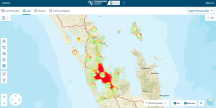
At the most basic level, the presentation of crash locations on a map can provide information on crash clusters. In the absence of a more sophisticated crash database system, this provides a quick indication of crash locations by frequency. Figure 10.9 shows an example of crash locations overlaid on a map for an urban area. In this figure the larger the circle, the higher the number of crashes. Maps are a powerful way to present information to key stakeholders, including technical staff, policy makers, senior managers, members of the public and politicians. As they are easy to understand by all of these stakeholders, they can be a strong advocacy tool. Another very useful tool in this regard are heatmaps, which make it possible to identify areas with a high number of crashes or fatalities or injuries based on the data shown.

CRASH FREQUENCY

Crash frequency is the simplest identification criterion. Each crash is located at its point of occurrence on the road network and the total number of crashes reported at each site being considered is added up. Sites are ranked in decreasing order of crash frequency.

A detailed safety analysis is warranted at each site where the crash frequency exceeds a selected investigation threshold (IT). This threshold may be set arbitrarily, e.g. although it should preferably take into account the available budget.

This approach allows the identification of a road site where the number of crashes is significantly higher than an established threshold value, which can be set arbitrarily, although it should preferably take into account the available budget. For example, a site with five or more crashes per year, or a road section with a crash frequency of 3 crashes per kilometre per year in a rural area might be classified as hazardous if the average crash frequency for the entire network is 2 crashes per kilometre per year.

The procedure and an example of application is shown in Appendix 10.2 (Crash Frequency).

Advantages

• Simplicity of the criterion.
• Sites with a high crash frequency are necessarily detected.
• Focus on crash reduction (collective risk).

Disadvantages (see box below)

• Bias towards high traffic volume sites.
• Does not take into account crash severity.
• Does not take into account the random nature of crashes.

More detailed information on this issue can be found in AASHTO Highway Safety Manual (2025) and Austroads (2021). These help in the identification of high-risk crash locations, particularly those of higher severity. It is important to note, however, that although high-risk locations should be targeted for treatment, they may only make up a small proportion of the network that is responsible for deaths and serious injuries. In these instances, additional proactive responses may also be required (see Section 10.4 Proactive Identification).

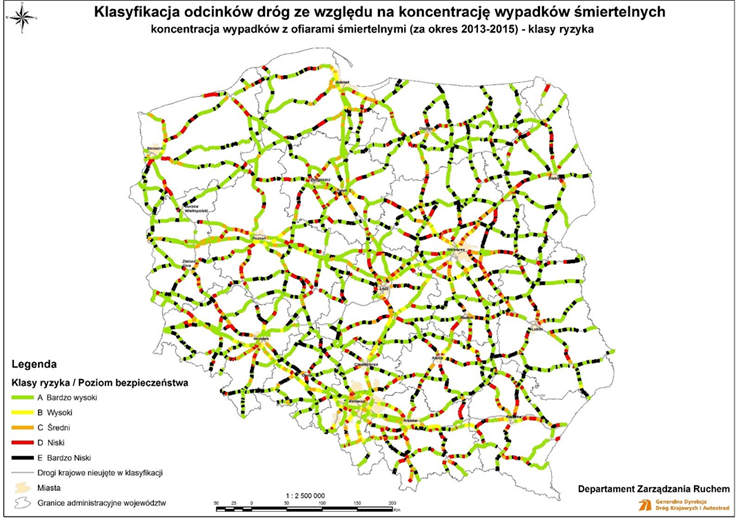
Figure 10.10 shows an example of road safety levels map based on fatal crash risk concentration for national roads in Poland. More detailed maps for smaller regions together with maps representing fatal crash acceptance risk levels, costs density class risks and costs density acceptance levels are also available. All the maps are prepared in accordance with polish national regulations (Dziennik Ustaw Rzeczypospolitej Polskiej, 2015) and European Directive 2008/96/EC on road infrastructure safety management.

CRASH RATE

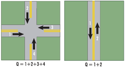
This approach identifies a site where the crash frequency is unusually high relative to its traffic volume. The crash rate, which is the ratio of crash frequency to traffic volume, indicates the level of risk exposure. Traffic volume is the most commonly used exposure unit (Figure 10.11):

• At road intersections (nodes), the traffic considered is the sum of entering vehicles.
• On road links, it is the sum of vehicles travelling in both directions. The length of the link must also be accounted for.

This criterion requires the definition of an arbitrary threshold for identifying high risk locations.

The procedure and an example of application is shown in Appendix 10.2 (Crash Rate).

Advantages

• Takes into account traffic exposure.
• Is the most widely used identification criterion, which facilitates comparisons.
• Focus on the probability of being involved in a crash (individual risk).

Disadvantages

• Traffic volume must be known at each site.
• Does not take into account the random nature of crashes.
• Bias towards low-traffic roads (a random variation of a few crashes per period will significantly modify the crash rate value at such sites).
• Does not take into account crash severity.
• Assumes a linear relationship between traffic volume and crashes; this may be a source of error.

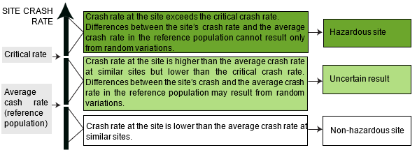
CRITICAL CRASH RATE

This criterion makes use of methods originally developed to conduct quality controls in industry (Norden et al., 1956). It compares the crash rate at a site with the average crash rate calculated in a group of sites having similar characteristics (see Appendix 10.1).

As for the other criteria described in this section, the basic assumption is that sites having similar characteristics should have similar safety levels. Despite this assumption and due to the random nature of crashes, a site's crash rate may very well exceed the average crash rate of its reference population without being necessarily hazardous. However, when a site's crash rate becomes too high compared to similar sites, random variations no longer suffice to explain the observed difference. The site is then considered to be deviant.

This criterion calculates the minimum crash rate value at which the site is considered hazardous.

The critical crash rate value increases with the chosen statistical level of confidence.

The procedure and an example of application is shown in Appendix 10.2 (Critical Crash Rate).

Advantages

• Takes into account the random nature of crashes.
• Takes into account traffic exposure.

Disadvantages

• Complexity of the method.
• Does not take into account crash severity.
• Assumes a linear relationship between traffic volume and crashes this may be a source of error.

This criterion, together with crash density, are also used in the reactive approach of the European Commission's Network Wide Road Safety Assessment (NWA) methodology for identifying high-risk locations (EC, 2023) based on the Directive 2008/96/EC as amended by the Directive (EU) 2019/1936.

EQUIVALENT PROPERTY DAMAGE ONLY (EPDO) INDEX

A common method of identifying high-risk locations to take account of severity is to prioritize sites through a crash cost analysis. An effective method often used is the Equivalent Property Damage Only (EPDO) Index, where crashes are weighted according to their severity. For instance, fatal crashes are assigned the highest cost/weighting per crash and property-damage-only (PDO) crashes (or minor crashes if PDO crash data is not collected) are assigned the lowest cost/weighting per crash.

The EPDO index attaches a greater importance to more serious trauma by ascribing to each crash a weight that is a function of the worst level of injury sustained by one of the crash victims. Thus, a crash causing minor injuries to two individuals and a serious injury to a third person is rated a serious crash. A crash that seriously injures two people has the same rating. Various weighting factors have been suggested in different countries, based on the social cost of crashes. Below an example of weighting factors proposed by Agent (1973):

• Property damage only crash (PDO): 1.
• Minor injury crash: 3.5.
• Serious injury or fatal crash: 9.5.

The procedure and an example of application is shown in Appendix 10.2 (EPDO).

Advantages

• Takes into account crash severity.
• Simplicity of the criterion.

Disadvantages

• Does not take into account traffic exposure.
• Does not take into account the random nature of crashes.
• Bias towards high-speed sites (rural roads).
• Does not take into account aspects not related to infrastructure or user behaviour (such as vehicle type and age, use of active and passive vehicle safety devices, etc.) for the severity of crashes.

The weighting factors attributed to each category of severity usually fall well below the actual cost of these crashes. The values recommended by Agent (1973) are still often used in North America. With similar values, greater but not disproportionate attention is given to more severe crashes.

The use of weighting factors that correspond to the real cost of crashes could lead to the underutilization of less serious crash data as it would take up to several hundred PDO crashes to equal one serious crash (Table 10.2). However, the repeated occurrence of crashes at the same location is a good indicator of road-related deficiencies that should not be overlooked, and the occurrence of a single severe crash at a location may very well not be related to prevailing road conditions.

* Note costs may vary by country and need to be current

RELATIVE SEVERITY INDEX (RSI)

This criterion is based on the following considerations:

1. The severity of trauma sustained in any given crash is affected by several factors, such as the impact speed, impact point on the vehicle, type of vehicle, age and health condition of the occupants, protection devices, etc. Consequently, two crashes of the same type occurring at the same location may cause quite different trauma levels.
2. The average crash severity, as computed on a large number of similar crashes having occurred in similar road environments, is seen as a more stable indicator than the trauma level sustained in a single crash.

Standard crash costs are assigned to crashes by crash type and road environment, as shown in the example in Table 10.3.

* Note costs may vary by country and need to be current

These costs are calculated based on an analysis of the average crash severity of each crash type. It is important to note, however, that crash types and crash costs will differ between jurisdictions and countries. This method takes into account crash severity but places less emphasis on locations where a single fatal crash may skew outcomes because of its very high cost. Such an outcome might be the result of a ‘random’ event, never to be repeated. This is more likely on lower volume roads or road networks where fatal crashes are very infrequent. Of higher interest are locations, routes or areas where high severity events are likely to happen again in the future. Using average crash costs by crash type, a crash cost can be assigned to each location, and then locations ranked by total crash costs.

The procedure and an example of application is shown in Appendix 10.2 (RSI).

Advantages

• Takes into account crash severity.
• Reduces the influence of exogenous variables having an impact on crash severity.

Disadvantages

• The development of the cost grid may be complex.
• Does not take into account traffic exposure.
• Does not take into account the random nature of crashes.
• Bias towards high-speed sites (rural roads).

COMBINED CRITERIA

In some cases, multiple identification methods are used. These use two or more of the methods identified above.

Various combinations of criteria can be used to reduce the shortcomings of individual criteria (Table 10.4).

For illustration purposes, three possible variants are described:

• Combined thresholds.
• Individual threshold.
• Individual threshold with minimum values.

Combined thresholds

• More than one investigation criterion is used to detect deviant situations, e.g. a crash frequency of 5 or more crashes per period and a crash rate of 3.0 or more crash/Mveh-km.
• All investigation thresholds must be reached in order for a site to be detected.

Individual threshold

• More than one investigation criterion is used to detect deviant situations, e.g. a crash frequency of 5 or more crashes per period and a crash rate of 3.0 or more crash/Mveh-km.
• A site is detected if at least one investigation threshold is satisfied, regardless of the value of the other criteria.

Individual threshold and minimum criteria values

• Sites are ranked in decreasing order of one criterion. Minimum investigation thresholds are set for the other criteria considered, e.g. ranking sites by crash rate and keeping only those sites with a minimum of 3.0 crashes per period.

The procedure and an example of application is shown in Appendix 10.2 (Combination of Frequency and Rate).

EMPIRICAL BAYESIAN METHOD

EB method is considered one of the most reliable approaches for selecting crash locations; that method provides a way to combine a site’s crash history with the crash history of several sites having similar characteristics (reference population) in order to calculate the site’s adjusted crash frequency (f_EB). This adjusted frequency is seen as a better approximation of the long-term average crash frequency on which safety decisions should be based. At first, the method of moments has been proposed to combine these two pieces of information, but multivariate statistical models are seen as a more practical method for this purpose.

The main problem associated with the use of empirical Bayes methods lies in the difficulty of defining homogeneous reference populations (Elvik, 1988). In order to overcome this problem, Hauer suggests using statistical regression techniques to develop crash prediction models (or ’safety performance functions’ – see Crash Prediction Models) that serve as reference populations. Details are explained in some Hauer's articles (Hauer, 1992, 2002, 2004), but the basic principles are as follows:

1. A multivariate statistical model (safety performance function), that relates crash frequencies to a set of independent variables, first needs to be developed and the value of the overdispersion parameter must be estimated during this development. This model is used to calculate a site’ s predicted crash frequency (f_pj).
2. The adjusted crash frequency at the site f_EB is computed by combining this predicted crash frequency (f_pj) and the number of crashes reported at the site (f_j). The relative weight attributed to f_pj and f_j is related to a weight parameter (w), as shown in [EQ. 10.1].

3. The value of ‘w’ is influenced by the relative homogeneity of the reference population that has been used to develop the statistical model (as expressed by the over dispersion parameter) and it is also influenced by the value of the number of crashes predicted by the safety performance (as this frequency increases, more importance is placed on the site crash frequency).

Advantages

• Takes into account the random nature of crashes.
• Improves the accuracy of the estimated potential for improvement.

Disadvantage

• Relative complexity.

CRASH PATTERNS

A road network’s safety deficiencies are usually identified by using one or more of the criteria described in Criteria for Selecting Locations to Investigate for Treatment. Such criteria detect crash concentrations, although the nature of the problems encountered is generally unknown at the time of identification. A complementary identification approach, which consists of searching for deviant crash patterns, may also be considered.

If a clear crash pattern can be found for which a cost-effective treatment is known, an action may be justified even though the overall crash frequency is not abnormally high. For example, a concentration of night-time crashes at a site may justify the installation of a road lighting system even though the overall number of crashes is not abnormal.

Given that the ‘normality’ is strongly influenced by the characteristics of the site being analysed, a comparison between crash features at the site and corresponding features at similar sites is recommended (see section Reference Population and Potential for Improvement in Appendix 10.1).

In order to identify deviant patterns with an acceptable level of confidence, the number of crashes considered must be sufficiently high. Consequently, this identification approach is more suited to the most frequent collision types, at locations where traffic volumes are high and for larger sites (route, area, network).

Various statistical techniques can be used to identify deviant accident patterns. The following paragraph describe how the properties of the binomial distribution can be applied to this end.

BINOMIAL PROPORTION

The properties of the binomial distribution can be used to calculate the probability of observing a number of crashes of a given type i at a site j(f_ij) when the total number of crashes at this site (f_j) and the average proportion of this type of crash in a population of similar sites (p_i) are known:

where:

f_ij = frequency of type i crashes at site j

f_j = total crash frequency at site j

p_i = average proportion of a type i crash in the reference population

Accordingly, the probability of observing fewer than f_ij crashes of type i at site j is:

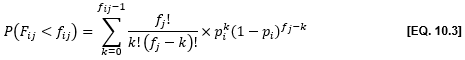
And the probability of observing f_ij or more crashes is:

When P(F_ij > f_ij) is low, the frequency of the type of crash under study is abnormally high.

The procedure and an example of application is shown in Appendix 10.2 (Binomial Proportion).

CALCULATOR: BINOMIAL TEST

CONCLUDING REMARKS

Crash sites can be assessed using statistical analysis to identify sites that are experiencing a statistically significant number of crashes in a set time period. This can be useful to distinguish between sites that are experiencing abnormally high crash rates and those that are merely experiencing variation due to chance.

Sites identified as hazardous may differ depending on which identification criterion is used. As mentioned previously, the crash frequency tends to detect more sites with higher traffic flows, while the crash rate detects more sites with lower traffic flows and crash severity detects more sites in rural environments. Each of them highlights problems from a different perspective and it appears as a good practice to analyse the safety performance of a road network from more than one angle:

• A high concentration of crashes at the same location is in itself a strong indicator of a road related problem that should warrant a safety diagnosis.
• The crash rate measures the level of risk faced by road users. When road users travelling at a specific location face an abnormally high risk, corrective actions should be taken.
• Reducing road fatalities and injuries should be the ultimate objective of any road safety action and accordingly, it is sensible to give special attention to those sites where more severe crashes occur, regardless of traffic.

The combination of empirical Bayesian methods and multivariate statistical models are seen as a more accurate and reliable method of identification of road safety problems (than traditional methods) as it reduces selection biases related to the random nature of crashes. While this increased sophistication might not be necessary when problems are obvious, which is likely to be the case in the early stages of road safety interventions, the application of these methods can be greatly facilitated by making a proper use of inexpensive computer technologies.

It should be recognized that other identification strategies can also be quite useful for detecting deviant sites:

• Detection of the worst sites of a road network, using the criteria described and ranking sites in decreasing order without considering the reference population to which they belong.
• Detection of a safety deterioration at a site between two crash periods; the Poisson test is recommended for this purpose (see Appendix 10.1 - Random Nature of Crashes).

CALCULATOR: POISSON TEST

The crash identification process allows for sites to be selected for further investigation. Using any of the abovementioned methods, a shortlist can be developed containing sites that will be considered for treatment. Available funding will limit the number of sites that can be treated, and so the shortlisted sites should be assessed through site inspections and an initial crash diagnosis to identify where cost-effective treatments can be implemented.

DIAGNOSING THE CONTRIBUTING FACTORS TO CRASHES

Diagnosing the contributing factors to crashes is the foundation for selecting an effective solution to a safety problem. To properly understand the problem, one must consider that:

• A crash is the result of a sequence of events and circumstances (rather than a single cause).
• Each event or circumstance is linked to a component of the Safe System – the persons involved, the vehicle, or the road environment.
• Each event is strongly influenced by the preceding event or circumstance.

Diagnosis of the contributing factors at a crash location is a four-step process:

• Gather the relevant information about the site, such as crash data, traffic volumes, and the history of the network or location in terms of land use or physical layout changes.
• Analyse the crash data for the location (e.g. the whole area if looking to perform mass action plans, or a single site for treatment implementation) by looking for common crash types or factors, particularly those that are happening in groups.
• Inspect the site from the perspective of the road user, and closely examine the site’s physical features and layout, understand the human factors and human behaviours that may be contributing to crash occurrence or outcomes.
• Based on the notes and findings from the above steps, draw conclusions about the likely contributing factors to the crash groupings (of similar type and/or location).

These stages are discussed in further detail in the sections below. The NCHRP Report ‘Diagnostic Assessment and Countermeasure Selection: A Toolbox for Traffic Safety Practitioners’ (National Academies, 2024) offers a valuable resource for diagnosing crash contributing factors and selecting appropriate countermeasures.

When conducting a diagnosis, analysts may have to consult technical references in order to better understand whether a road component can contribute to a given safety problem or could improve the situation. Technical Sheets describe the relationship between several road features and safety (horizontal alignment, vertical alignment, intersection, etc.). Some technical data may also need to be collected at the site to make progress in the diagnosis. Technical Studies explains how to conduct various technical studies: spot speed, traffic count, etc.

Results obtained at each of the abovementioned four steps may be closely related. For example, a safety deficiency at a horizontal curve is likely to be detected during both the crash analysis step (large proportion of single-vehicle crashes) and the site observation step (isolated sharp curve). In other cases, the conclusions of each step will be complementary. For example, the crash analysis may detect a cluster of nighttime collisions, which will focus the analyst’s attention on problems that may not have been detected by a daytime field survey. It is therefore highly recommended to complete all the steps of the diagnostic process, even when a solution seems to have been found at the beginning of the analysis.

Given that each site has its own combination of road characteristics, road users and vehicles, the list of potential safety problems and relevant solutions is quite long. When conducting a safety diagnosis, the analyst should verify the following points:

• The differences between the site features and established standards or practices.
• The complexity of the driving task and the compliance with drivers’ expectancies.
• The coherence of the road environment

Sometimes, desirable actions may extend beyond road engineering work. The range of measures that may be implemented to improve safety is quite wide. It should be clear that the realization of a safety diagnosis requires knowledge not only in road engineering, but also outside this field (human factors, vehicle engineering, statistics, etc.). The analyst has to determine whether the most appropriate treatment is related to the road or to other components of the safety system.

The analysis of complex cases for which there is no obvious solution requires the contribution of a multidisciplinary team of experts who together are more likely to develop a good understanding of the problems encountered and to propose appropriate solutions. Accordingly, it is important to ensure that efficient coordination structures and communication channels are developed between the main groups playing an active role in road safety, in order to allow constructive interdisciplinary exchanges leading to the implementation of optimal solutions.

From the standpoint of road safety engineering, it is also important to keep in mind that problems may originate at different stages of development and operation of a road network: planning of the transportation system, road designing, construction, operation and maintenance (some examples are listed on the next page).

The ability to make a good safety diagnosis is therefore highly related to the experience and ‘sound engineering judgment’ of the analyst who, after having conducted several of these studies, will know how to recognize situations that increase the collision risk. Obviously, this is a knowledge that cannot be learned only from textbooks, but the process described in this section should help those with less experience in gaining a better understanding of the underlying principles and logic of their work.

GATHER RELEVANT INFORMATION

Crash data is the most important information and should be available from either the Police or road authority or leading road safety agency. The road agency may also have information on traffic volumes and any historical information about the site such as a layout plan, any changes in traffic patterns or land use, and any previous or current concerns raised by the community or stakeholders.

All this information should be gathered and analysed at the beginning of the diagnosis to:

• Be informed of problems identified in the past and actions taken.
• Avoid duplication of effort - if no major change has occurred at the site, some technical studies may not have to be repeated.

ANALYSE DATA

The analysis of the available crash data is a fundamental step of a safety diagnosis as it helps in gaining a better understanding of problems that have been experienced by road users travelling at the site. As a result, analysts can propose solutions that are well suited to encountered problems and will help in reducing the occurrence of similar crashes in the future.

The crash analysis should be initiated prior to the site visit as it may influence observations that need to be made at the site. In some cases, analysts will also have to bring additional equipment, to verify the relevance of potential accident factors (speed gun to measure operating speeds, rods and measuring wheel to determine available sight distance, etc.). Accident tables should be brought to the site (Appendix 10.3).

UNDERSTANDING THE CRASH

To properly diagnose safety problems, an analyst must first have a good understanding of the crash mechanisms:

• A road collision is the end result of a sequence of events occurring under specific circumstances (rather than the ‘cause’ of a single factor).
• Each event and each circumstance are linked to one of the three basic components of the safety system - human, road environment, vehicle.
• Each event is strongly influenced by the result of preceding actions and circumstances of these actions.

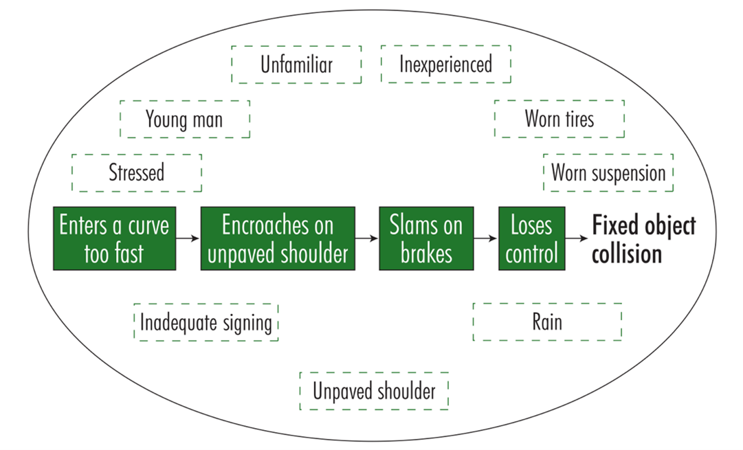
The following example illustrates a hypothetical crash sequence:

An 18-year-old man who had his driving licence for six months was going for a job interview in an unfamiliar area. He was late, tense and speeding. It was raining. His vehicle's suspension and tires were worn. At the approach to a sharp curve after a long, straight section, he did not see the warning sign, which is deficient under prevailing standards, and entered the curve too fast. He encroached on the shoulder, which was unpaved, slammed on the brakes, lost control and collided with a tree by the side of the road.

Analysts must seek to understand such chains of events and circumstances leading up to each crash in order to propose measures that may break these sequences (Figure 10.13). Where there is not enough information to reconstruct the course of each crash in detail, simplified analysis methods must be used.

CRASH ANALYSIS LEVEL

Different types of analysis levels can be recognized based on the number of crashes considered:

• The micro level, where a single crash is analysed. Typically, this analysis is conducted after a serious crash, to accurately reconstruct its chain of events and circumstances.
• The intermediate level, where all crashes having occurred at a same location with a poor safety record are analysed to find solutions that will reduce their future occurrence. The diagnosis process described in this section is best suited to this level of analysis.
• The macro level, where a larger set of crash data is considered. It may be the set of all crashes on a road network, all crashes involving a specific type of road user (pedestrians, heavy vehicles), or all crashes on a given road category. Results of macro-analyses conducted on road categories may yield useful information when conducting a safety diagnosis at a specific site, by providing insight into problems that are likely to be encountered. Such analyses are also conducted when developing a country’s road safety action plan and establishing a country’s action priorities (see Chapter 6. Road Safety Targets, Investment Strategies, Plans and Projects).

STATISTICAL CRASH ANALYSIS

Typically, crash reports contain several elements of information that may highlight potential road deficiencies (Table 10.5).

By combining information from the collision report, the analyst may sometimes obtain results that are similar to quasi-scenarios: heavy vehicle on grade; right-angle collision at intersection at rush hour, etc.

Additional information contained in the collision report may also reveal problems that require actions on other components of the ‘human – environment – vehicle’ system: impaired driving, young drivers, overloaded vehicles, mechanical defects, etc.. In such cases, the appropriate authorities should be informed of the existence of the problem.

Steps of a statistical crash analysis are as follows:

1. Preparation of crash summaries. Various crash summaries can be prepared to help identify abnormal crash patterns. Below, three types of summaries are described: Collision diagrams, Factor matrices, and Comparative tables.
2. Search for contributing factors. Once deviant crash patterns have been identified, the analyst will seek to understand their causes (contributing factors) in order to determine whether road engineering actions could efficiently prevent similar crashes in the future. The first part of the Crash Tables in Appendix 10.3 provides practical assistance in this task. Separate tables have been developed for nodes and links and for the most frequent accident types.
3. Search for solutions. For each crash contributing factor, there are generally several actions that can be envisioned to improve the situation. The second part of the Crash Tables in Appendix 10.3 lists the most common treatments.

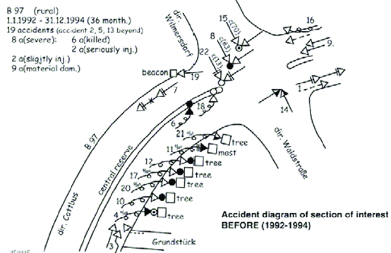
COLLISION DIAGRAM

A collision diagram is an illustrative presentation of the crashes that have occurred at a location. Crashes are pinpointed on a diagram of the intersection or road section, showing the crash type (through standard symbols), the direction of travel, and other relevant information (e.g. the date, time of day, weather and lighting conditions). A number of software packages allow the automatic creation of these diagrams.

The main purpose of these data presentation types is to identify common contributing factors of crashes at a location. Note that there are normally several factors that lead to a crash. If there is no apparent dominant crash type that appears from the data, it can be very difficult to treat the site as it will be difficult for anyone treatment to solve all the different issues at the site (speed management can be the exception to this, particularly in the elimination of high severity crash outcomes). Often it can be helpful to look at the individual police crash reports for greater detail on the crash circumstances, as this might shed light on a common causal factor.

FACTOR MATRIX

A factor matrix takes the frequency table approach one step further and considers additional factors such as the crash severity, year of the crash, direction of travel, type of road users, collision type, surface and lighting conditions, time of day, and day of week. A key aspect of the factor matrix is the inclusion of the movement code or ‘stick diagram’ to indicate vehicle movements in each collision.

COMPARATIVE TABLES

What constitutes an abnormal proportion of crashes depends greatly on the site category being analysed. For instance, average proportions of rear-end collisions or right-angle collisions at an intersection will depend on whether the right-of-way is managed by stop signs or traffic signals; the proportion of run-off the road crashes is higher on horizontal curves than on straight alignments, etc.

Therefore, comparing crash patterns at the site under study with crash patterns at sites having similar characteristics (reference population) will help provide a more accurate estimate of the anticipated improvement potential. For example, Table 10.6 shows that in this dataset, a 40% proportion of rear-end collisions is below average at an intersection with traffic signals, but above average at an intersection with stop signs.

TABLE 10.6: EXAMPLE – CRASH PROPORTIONS AT 4-LEG INTERSECTIONS

TRAFFIC SIGNAL	45%	30%
STOPS	32%	48%

However, it is first necessary to ensure that the geometric and traffic characteristics of the reference population are adequate; otherwise, this comparison might simply lead to the maintaining of unsafe conditions. Appendix 10.1 discusses this problem in greater detail.

Various statistical tests can be used for this comparison and Section Crash Patterns describes how to calculate binomial proportions to this end. Table 10.7 shows the results of this calculation for the variable ‘vehicle type’. In this example, the high proportion of crashes involving a heavy vehicle requires more in-depth investigation.

SITE/ROUTE/AREA INSPECTION

The main purpose of an inspection is to identify any environmental or traffic issues that may be contributing to crashes at the location. A site inspection can allow the crash investigation team to see the location through the eyes of the road user and observe the traffic behaviours. Additional data can also be collected, such as vehicle speeds, road features, parking restrictions and speed limits, as well as enable the team to assess any other characteristics of the surrounding road environment.

Where possible it is recommended that a team conduct the assessment, rather than an individual. A team approach will generally provide a more diverse range of opinions and ideas, as it is easier to generate these through group discussion. Team members might include an expert who is trained in road safety engineering and investigation of crash locations; and police and/or road agency staff, particularly those who are familiar with the location. The group may also include someone new to the crash investigation, but who has ideally undergone some form of training. This approach is essential to ensure development of skills for future crash investigators. Guidelines on Human Factors should be considered by those investigating sites (see Chapter 8. Design for Road User Characteristics and Compliance, and National Academies, 2024)

Table 10.8 provides a list of possible contributing factors for different crash types (including those that contribute the most to fatal and serious injury outcomes) that should be considered by investigators during a site inspection. Although not listed, speed is linked to the frequency and severity of all crashes.

FIELD PREPARATION

The analyst must bring to the site the following items:

• Crash tables (Appendix 10.3).
• Diagnostic checklists (Appendix 10.4)
• Video camera with integrated GPS and with sufficient recording media and batteries.
• Measuring tape and measuring wheel.
• Paper, pencils, ruler, and eraser.
• Smart phone.

When available, the following should also be brought to the site:

• Road drawings (geometric design, signing, marking, lighting, etc.).
• Reports of previous studies (to verify whether problems identified in the past have been corrected as recommended).
• Conclusions of the crash analysis.

It may also be helpful to provide the following items (particularly if the site is far from the office):

• Sighting and target rods (Sight Distance study).
• Speed gun (Spot Speed study).
• Stopwatch (Travel Time and Delay, traffic-signal timing).
• Tally sheets or mechanical or electronic counter (Traffic Count).
• Tape recorder.
• Level (superelevation).

For the analysts’ safety, also provide:

• Reflective vest.
• Safety helmets and boots (when necessary, e.g. in a work site).
• Rotating beacon and other required road signalling equipment.
• Police assistance (when necessary).

SITE FAMILIARIZATION

The main objectives of the site familiarization are to detect obvious problems and to understand the main difficulties encountered by drivers at the analysed site. Upon arrival, the analyst drives through the site at the same speed as other drivers and in all permitted directions. The distance to be covered depends on the type of road environment and the nature of the suspected problems. In urban areas, a distance of a few hundred meters in each direction is usually sufficient. In rural areas, the distance to be covered may be much longer and extend up to several kilometres when the problem may be related to a violation of drivers’ expectancies. The analyst must also complete pedestrian manoeuvres.

While driving along the road, it is useful to record a geolocalised video from the vehicle. This allows the team to watch the video at a later stage and capture details that may have been lost during the site visit. It is often useful to select someone unfamiliar with the area to do the driving so that they can experience the location as others would for the first time. Often there will be a need to drive through the site several times. Sometimes it is also useful to inspect the site at different times of the day or days of the week to check for any variability in traffic flows or lighting/visibility conditions. For example, if a high number of night crashes have occurred, night inspections are essential.

Various types of problems can be detected during the site familiarization:

• Hazardous road or roadside characteristics (restricted sight distance, inadequate signing, hazardous roadside conditions, etc.)
• Hazardous traffic conditions (severe traffic conflicts, high speed differentials, excessive delays etc.)
• Risky behaviour (poor compliance with traffic, rules, excessive speeds, tailgating, etc.)
• Expectancy violations or inappropriate driving task requirement (inadequate transition zone, multi-branch intersection, etc.)
• Obvious coherence problem (commercial stand on highway shoulder, non-local traffic on residential street, etc.)
• Insufficient maintenance (faded markings, worn road signs, overgrown vegetation, etc.)

DETAILED OBSERVATIONS

At this stage, the analyst:

1. Makes observations related to problems that have been found in the previous steps of the diagnosis, i.e.:
   • Verifies whether problems that have been identified in the past at this site have been successfully treated.
   • Completes the determination of possible crash contributing factors and potential solutions.
   • Analyses problems that have been detected during the site familiarization.
2. Checks whether problems that are frequently encountered at similar sites are also found at this site.
3. Observes traffic conditions. Excessive delays and travel times may cause road-user frustration, leading to risky behaviour, such as short gap acceptance, tailgating or illegal passing manoeuvres. If these problems are observed or suspected, a more detailed analysis of the traffic conditions should be conducted. This will always include a traffic count and a capacity analysis, and, in some instances, additional technical studies may also be required. The analyst should also ensure that no category of road user has an unacceptable level of risk. Frequent problems include:
   • Hazardous left-turn manoeuvres on high-speed roads (insufficient protection).
   • High speed differentials (between road users at the same location or for the same road user between two road segments).
   • High mass differentials (inappropriate mixes of road users sharing the road).
   • Severe traffic conflicts.
   • Encroachments (e.g. during turning manoeuvres of heavy vehicles at intersection).
   • Inadequate consideration of the needs of specific categories of road users (e.g. audible crossing signals for blind people, longer crossing times for elderly persons, etc.).
4. Makes detailed observations of the features of the road environment (land use, speed, horizontal and vertical alignment, sight distance, cross-section, road surface conditions, traffic signs and markings, roadside conditions, accesses and crossings, road lighting, intersections features, etc.). Analysts should verify that each of the features follows relevant standards or practices and assess the associated risk when deviations are observed.
5. Assess drivers’ workload and expectancy violation. If needed, a more detailed analysis of the driving task should be conducted.
6. Check whether road safety problems may be linked to inappropriate road user behaviour and determine if such behaviour could be efficiently prevented by changing some road features. When the problem would be better solved by other types of actions (e.g. education, enforcement), contacts should be made with the agencies responsible to ensure that they are well aware of the problem.
7. Check whether the safety problems may be related to inadequate maintenance. Frequent deficiencies include worn road signs, faded road marking, overgrown vegetation, distressed road surface, damaged road safety equipment (e.g. guardrails) and broken road light or traffic signal.

To ensure a comprehensive analysis, most of the above work will be performed on foot, which will also allow for thorough photographic and written documentation of all inspection observations and findings.

DRAW CONCLUSIONS

Before summarising the analysis in a report, consideration should be given to whether any additional information is required. For instance, if the crash analysis and/or site inspections suggest that there may be issues with skidding, then skid resistance testing could be undertaken.

A summary report should be prepared to clearly inform readers of the conclusions that were drawn from the analysis. This provides the basis from which treatment options are considered and selected. The report should include a description of the area or site, results from the data analysis (e.g. crash diagrams), observations from the site inspections, including possible contributing factors to crashes, comments on any identified common factors leading to crashes and possible remedial measures (see Section 11.3 Intervention Options and Selection).

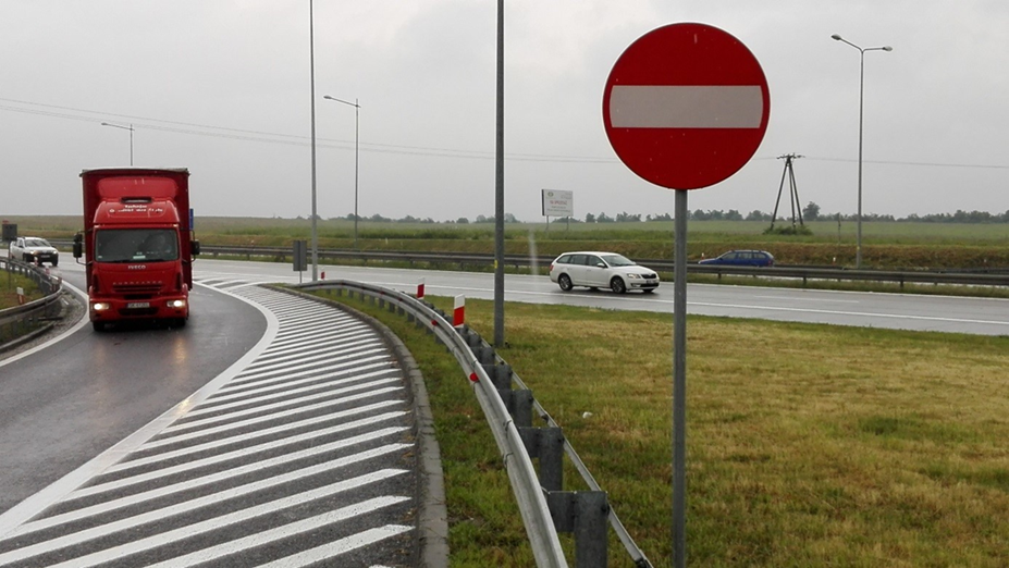
As an example of a diagnosis, on motorways and expressways wrong-way drivers (or ‘ghost riders’) were occasionally identified. The road authority recognised that the design should limit the possibility to travel the wrong way on roads where the opposite directions are physically separated. Some of the engineering solutions that were implemented long ago, were no longer recommended, but still exist and operate well when properly equipped with traffic signs and markings. Ghost riders were also identified on new roads. After specially dedicated inspections with road traffic specialists and police, some additional signs minimising of the potential of unintentional wrong-way driving were installed. Solutions were adapted and placed on other new and existing roads as shown in the photo above. These actions removed the need to rebuild. This solution is used on new investments with practically zero additional costs.