


APPENDIX 12.1 – STATISTICAL TESTS
STUDENT t-TEST – COMPARISON OF SAMPLE MEANS
To determine whether the mean speed of a set of speed measurements is significantly different from another (i.e. between a before and after study), it is appropriate to use Student two-tailed t-test, making the reasonable assumptions that the variances of the two sets of measurements are drawn from the same population. The null hypothesis is thus that there is no difference in the means (i.e. that drivers’ speed has not been affected by the scheme). It is first necessary to determine the standard deviation of the difference in means. We then calculate the equations below:
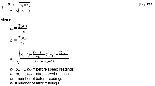
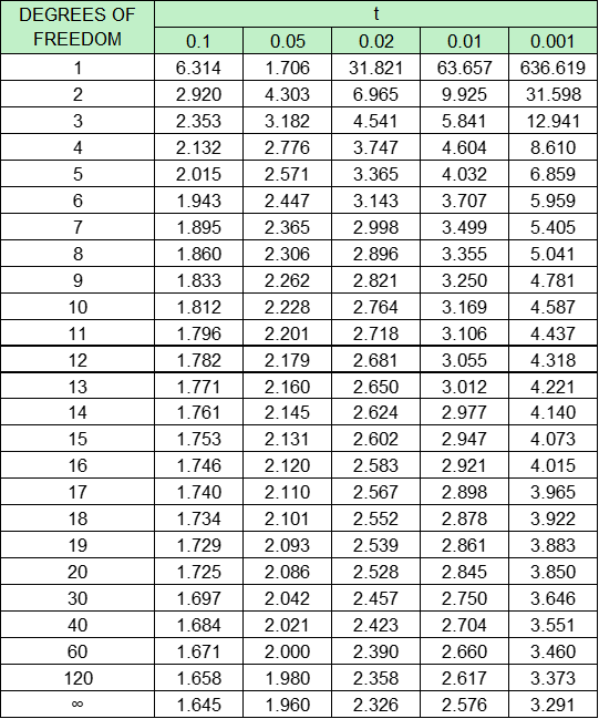
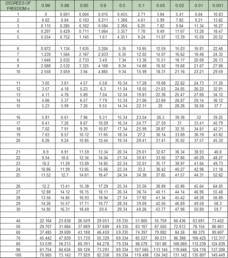
Having calculated the value of t, we need to look at a table of Student t values (Table 12.A1) with (na + nb – 2) degrees of freedom (ʋ). If the calculated value of t exceeds that for the 5% level (the t = 0.05 column), we can be 95% confident that the true mean speed has changed.
Example
Assume that the following results were obtained from spot speed studies:
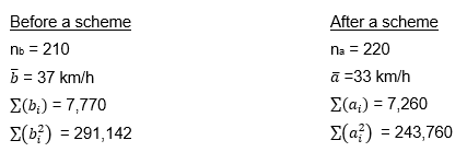
From equation [EQ. 12.1]:
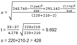
As the calculated t value (9.69) is greater than 1.96 (large number of degrees of freedom), we can say that the difference in mean speeds (a 4 km/h reduction) is significant at the 5% level.
This test can be conducted with the CALCULATOR: DISTRIBUTION TEST
TABLE 12.A1: TABLE OF T-DISTRIBUTION
KOLMOGOROV-SMIRNOV TEST
The ‘two-tailed’ test determines whether two independent samples have been drawn from the same population (or from populations with the same distribution). In some cases, two data sets may have the same mean but different dispersion, which may be the cause of safety problems. If the two samples have in fact been drawn from the same population (the null hypothesis), then the cumulative distributions of both samples may be expected to be fairly close to each other, i.e. they should show only random deviation from the population distributions. If the two sample cumulative distributions are too far apart at any point, this suggests that they come from different populations. Thus, a large enough deviation between the two sample cumulative distributions is evidence for rejecting the null hypothesis.
Let SNa(x) be the observed cumulative step function of the first speed sample: i.e. SNa(x) = K/Na where K is the number of vehicles equal to or less than x km/h and Na is the total number of vehicles of the sample. Let SNb(x) be the cumulative step function of the second sample. Now the Kolmogorov-Smirnov two-tail test focuses on the maximum deviation, D.
For large samples (N > 40), Kolmogorov-Smirnov tables show that the value of D must equal or exceed the following value to reject the null hypothesis at the 5% level, i.e. they are not from the same population:

The ‘one-tailed’ test determines whether the two samples have been drawn from the same population or whether the values of one sample are stochastically larger than the values of the population from which the other sample was drawn. The maximum deviation is again calculated using [EQ. 12.2] and the significance of the observed value of D can be computed by reference to the chi-square distribution.
It has been shown that for large samples, the following statistic has a sampling distribution that is approximated to the chi-square distribution with two degrees of freedom. The chi-square table is given in Table 12.A2.
TABLE 12.A2: TABLE OF X2
k TEST
The k test can be used to show how the crash numbers at a site have changed compared to control data.
For a given site or group of similarly treated sites, we have:
where:
a = before crashes at site
b = after crashes at site
c = before crashes at control
d = after crashes at control
If k < 1 then there has been a decrease in crashes relative to the control.
if k = 1 then there has been no change relative to the control.
if k > 1 then there has been an increase relative to the control.
If any of the frequencies are zero, then ½ should be added to each, i.e.:

The percentage change at the site is given by:
Example Table 12.A3 shows the annual injury crash totals for a T-intersection in a semi-urban area that had stop signs on the minor road originally, but where a roundabout was installed three years ago. The control data used are crashes on all other priority intersections in the district over exactly the same 3-year before and 3-year after periods. TABLE 12.A3: INJURY CRASH FREQUENCIES AT TREATED SITE AND CONTROLS
Using the notation and equation above: Therefore, as k < 1, there has been a decrease in crashes relative o the controls of: (k-1) x 100% = 68% This test can be conducted with the CALCULATOR: BEFORE – AFTER TESTS (INDIVIDUAL SITE). |
THE CHI-SQUARE TEST
This test can be used to determine whether the change in crashes was produced by the treatment or occurred by chance. The test thus determines whether the change is statistically significant. It is based on a contingency table showing both the observed values of a set of data (O) and the corresponding expected values (E). The chi-square statistic is given by:

Where:
Oij = the observed value in column j, row i of the table
Eij = the expected value in column j, row i of the table
m = the number of columns
n = the number of rows
A chi-square table is then used to look up this value, which shows the probability that the ‘expected’ value and the ‘observed’ values are drawn from the same population. The number of degrees of freedom is also required and this is given by:
Degrees of freedom (ʋ) = (n – 1) (m – 1)
For a site crash evaluation, where its crashes are compared in similar periods before and after treatment with a set of control sites for the same periods, we have a 2 by 2 contingency table (2 columns and 2 rows with degrees of freedom = 1). For the test to be valid, the value of any cell of the table should not be less than 5.
Using notation from Table 12.A3, the chi-square value can be calculated by the following equation:

This value is then compared with the chi-square values in Table 12.A2 with degrees of freedom, ʋ = 1, and if it is greater than a particular value, it is said to be statistically significant at least at that percentage level.
Example Using the data in the previous example and the [EQ. 12.9], we obtain: 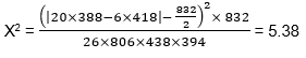 Now looking at the chi-square distribution table (Table 12.A2) and the first line (one degree of freedom, ʋ =1), the value for chi-square of 5.38 lies between 3.84 and 5.41. This corresponds to a value of significance level (on the column header line) of between 0.05 and 0.02. This means that there is only a 5% likelihood (or 1 in 20 chance) that the change in crashes is due to random fluctuation. Another way of stating this is that there is a 97,9% confidence that a real change in crashes has occurred at the intersection. The 5% level or better is widely accepted as indicating the remedial action has certainly worked, though the 10% level can be regarded as indicating an effect. |
GROUP OF SITES WITH THE SAME TREATMENT
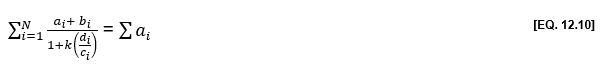
For a number of sites, N, which have had the same treatment, determining the overall effect requires a rather more complex calculation, i.e. by solving the following equation for k over all the sites, i.e. i = 1 to N. The other symbols are as in previous equations.
For testing, the natural logarithm of a variable such as is usually found to have a more symmetrical distribution (amenable to standard statistical treatments) and the standard error of loge k can be approximated to the following:
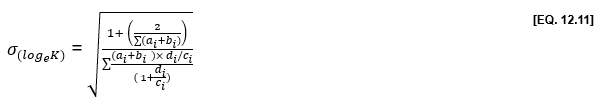
The following ratio should then be calculated using loge of the value of k calculated above and its standard error from the previous expression:

And if this value is outside the range ±1.96 (Student t), then the change is statistically significant (at the 95% level).
Now to test whether the changes at the treated sites are in fact producing the same effect on crash frequencies, we need to calculate the following chi-square value.

If this is significant with N-1 degrees of freedom (refer to the (N-1)th row in the chi-square table, where N is the number of treated sites), then the changes at the sites are not producing the same effect. If it is not significant, however, then it is likely that the changes are producing the same effect.
CALCULATOR: BEFORE – AFTER TEST (GROUP OF SITES)
REGRESSION TO THE MEAN CORRECTION
To correct for the regression-to-mean effect, the safety level (or long-term average crash frequency) must be estimated. Several statisticians have proposed ways of doing this. For example, Hauer (1992) recommended using Empirical Bayesian method to estimate the level of safety of a site and then use this value in safety studies (rather than the raw data). However, Abbess et al. (1981) previously described a simpler approach for a single site, in which the data was adjusted to correct for biases using assumptions about the distribution of crashes over a period of years.
Crashes data must be gathered for sites that are similar to the treated site over the same time period. Using this full dataset, the mean number of crashes, a, and the variance of crashes, m var (a), are calculated. The regression-to-mean effect, R (in %), is given by the following equation:

where:
A = number of crashes at the site
n = number of years
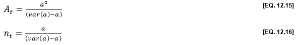
At and nt are the estimates of the parameters of the statistical distribution showing the true underlying crash frequencies, i.e. the crash frequency’s probability distribution before any data is available. The main assumption is, therefore, that the study site with a particular crash history will behave in the same way as the set of all similar sites with the same crash history.
Example Let us consider an intersection that has had an average of 15 crashes per year over the past 5 years. The site was widened, large new intersection signing, splitter islands and STOP signs were installed, after which the site has averaged 10 crashes per year over a similar period. To correct for the regression-to-mean effect, we need to select similar uncontrolled intersection sites with similar traffic flows. If all these sites have produced a mean, a, of 12.6 crashes per year with a variance, var (a), of 2.91, the input values are: a = 12.6 crash/year var(a) = 2.91 (crash/year)2 A = 75 crash/5 years n = 5 years At = 12.62 / (2.91 – 12.6) = –16.38 nt = 12.6 / (2.91 – 12.6) = –1.3 Thus, the regression effect: In other words, during the after period we would expect that if nothing were done to the site, the crashes would drop by 5.6%, or to 14.16 crashes per year. Thus, it is the figure of 14.16 crashes per year that should be compared with the 10 crashes per year that actually occurred to determine whether the reduction in crash frequency due to the improvements is statistically significant. |